Forecasting Actuarial Waiting Times for Accidental Nuclear Winter#
dv_ClaOp55Max_OOv4r4p1_2026m09d24_12h32Broader Significance
Nuclear war is usually argued in words. This study argues it in numbers, using the oldest quantitative discipline built for questions of this shape: actuarial science. An actuary cannot say when a particular person will die. Given a population, a set of risk factors, and a claims history, an actuary can still price the risk — and be wrong in ways that show. This study treats the system of nuclear-armed states as the life being priced, the Cold-War record of near-misses as the claims history, and accidental nuclear winter as the death.
At the rate crises have actually arrived, half of all runs of world history reach accidental nuclear winter within about twenty years, and the chance it begins in any given year is worse than one in forty. Set beside a risk that societies accept without alarm — dying in a road accident — a person is more than fifty times more likely to die as a consequence of accidental nuclear winter than in a car crash, counted the same way: annual, per person, death against death. That comparison is this study’s central claim, and it is built to be attacked rather than admired. It survives when the most sceptical published reading of the record, the lowest published death toll, and the road-death rate of the worst-affected country on record are applied all at once.
This risk is not invisible because it is small. It is invisible because it has been removed from the places where risks are measured. Nuclear war is excluded by standard clause from essentially every insurance policy written: the profession that prices catastrophe for a living examined this one and declined it, on the correct grounds that it is uninsurable in principle — there is no surviving counterparty to pay. It was priced at infinity, and then not spoken of. What follows is not alarm. It is arithmetic, from public data, repeatable in an afternoon.
A second calculation, which does not depend on the first being right, asks the question backwards: not how large the danger is, but how small the prospect of success may be before paying to attempt a remedy is still worth doing. Priced against a remedy costing about eight dollars a person a year, the answer is on the order of one in a few thousand — and stays at no more than three and a half percent even if this study has overstated the danger by a factor of a hundred. A reader does not have to accept the forecast in order to accept what follows from it.
Readers who suspect this of being alarmism should go straight to the strongest published objection (SIA-11): the most sceptical published critic of nuclear close-call analysis supplies this study’s own optimistic scenario, and the conclusion holds there too. Readers who want the argument without the theology will find it in a companion written in entirely secular terms.
The study is offered not to be believed, but to be checked. If it is wrong, the fastest way to find out is for someone to say so. #AuditTheMath
Declarations
Abstract
How long does a civilization survive with nuclear weapons and without periodic recalibration? This paper answers the way an actuary prices a life — as a probability distribution over time-to-failure, calibrated on a claims history and falsifiable against it. RiskyMAD is a three-state model (Risky / MAD crisis / Dead, the last absorbing) with one rate that must come from the world: the crisis rate, counted from the sixty near-misses catalogued by Baum, de Neufville and Barrett (2018) at about 0.1 per year; the chance a crisis escalates is taken, unmeasured, as one in three. The result: half of all runs over within about twenty years, an annual probability worse than 1 in 40, and more than 70 percent over a forty-year career — for most people, a likelier death than a car crash, by a margin that survives every scenario. Every figure in this paper’s body is stated as a bound that under-claims, with the exact values kept in the appendices. The result is a decision, not only an estimate: it is invariant across the full range the record can bear, and only a crisis rate of exactly zero — which no one claims — would overturn it. Because the Dead state is absorbing, onset is a stochastic certainty under business as usual; the only open question is when. The mechanism is a saturating two-step process, so long quiet stretches are exactly what the model predicts most of the time — which is why eighty-one quiet years are weak evidence, not reassurance. A candidate escape, MAP, is derived and priced by the same model, and then priced a second way that does not need the forecast to be right: asking not how large the danger is but how small the prospect of success may be before paying to attempt a remedy is still worth doing, the required probability comes out on the order of one in a few thousand, and stays at no more than three and a half percent even if this study has overstated the danger a hundredfold — rising to a real hurdle only for a reader who also holds one person’s whole stake in the world to be worth almost nothing. What is new here is narrower than the subject. Quantitative estimation of nuclear-war risk is an existing literature, and this study’s headline figure corroborates rather than displaces it. What it adds is the exact first-passage law in place of a Poisson shortcut; the whole distribution in place of a point estimate; the Michaelis–Menten correspondence as an identity rather than an analogy; the survival of the mean without the exponential assumption; and an identifiability result fixing what the record can and cannot separately estimate. That this gap was open is not asserted here but cited: Baum (2018) lists precisely this quantification among the things still to be done. SIA-10 sets out each claim and its nearest published relative.
Every input is public and every step is open to inspection. Don’t believe it — #AuditTheMath.
1. Introduction to the Question#
October 1962: Vasili Arkhipov and the meaning of nothing
On 27 October 1962, the most dangerous day of the Cuban Missile Crisis, the Soviet submarine B-59 lay pinned beneath a United States Navy hunting group that did not know she carried a nuclear torpedo. Her cooling had failed, her air was running out, and the practice charges dropped to tell her to come to the surface sounded below like an attack. For days nothing had come in from Moscow, and that nothing fitted two worlds equally well: no war yet, or Moscow was already wiped out, with nobody at the far end of the radio. Her officers could stay down and suffocate, fight their way out with a weapon of last resort, or surface into the arms of the enemy. Twice that day the captain reached for that nuclear torpedo. Below, he ordered the nuclear torpedo readied, convinced his patriotic duty demanded its use. Yet Vasili Arkhipov spoke up against a furious captain, in a boat that might already be at war, and — by the one witness’s account — talked him out of it [Savranskaya, 2005]. So the captain decided to surface instead. No available evidence could settle which world they were in. What Arkhipov said is not recorded, but only one line of reasoning fits what he achieved: the asymmetry of being wrong about what that “nothing” meant. He argued otherwise gently, kindly and reasonably, and it was convincing enough to move the captain to surface into the arms of the “enemy”: Firing their last remaining “super-weapon” would ignite or escalate the war they all hoped to prevent (a horrendous long-term cost), yet surfacing needlessly would in the worst case personally cost them their submarine, their career, and likely their lives - a huge personal cost they deemed worth paying for a shot at securing the long-term common good of keeping the world out of a global nuclear war. After surfacing the captain was blinded by powerful searchlights. He ordered an urgent dive and tubes 1 and 2 readied to fire with the nuclear torpedo in tube 1. Arkhipov saw that the American ship was signalling by lamp, not attacking, and cancelled the dive — another gentle, kind, reasonable call. Then the ambiguous semantics of nothing (ASON) displayed its benign side: The disaster the crew had feared did not happen as the nothing of “not yet” did not turn into the nothing of “no more” (for this MAD crisis). This moment and others like it in effect won WW3 for everyone, friend and foe alike, because there are no winners in a global nuclear war, only losers. And so WW3 became known as the Cold War, because no hot escalation has happened yet. Unfortunately, many oversimplify the wrestling with the complexity of a global nuclear machinery into concluding that “nothing” happened and that heroic acts of logical reasoning for the common good as done by Vasili Arkhipov do not need celebrating on a dedicated day of remembrance. Hence, instead of moving on, such a nihilistic view of nothing binds the world into a status quo that will keep waiting for a hot WW3 until it arrives, because it fails to see how the WW3 was already won for everyone. That is how forgetting tends to contribute to the arrival of accidental nuclear winter by perpetuating the status quo of nuclear roulette. More details of Arkhipov’s story are in Supporting Information Appendix SIA-X7. The rest of this study explores how often near-disasters like this one have occurred so far, what that is saying about a complex system like our world, armed with enough hair-trigger nuclear weapons to blow itself up, and how all these insights can be combined into a probabilistic model for predicting waiting times until a globally devastating nuclear war will occur by accident. Not because anyone wants to, but simply because eventually some battle station somewhere will not have someone like Arkhipov around to offer a gentle kind reasonable alternative for how to best interpret observations that seem to be “demanding” the use of nuclear weapons.
Which raises the question this paper exists to answer.
How long does a civilization with nuclear weapons survive without periodic rebalancing?
This is not a philosophical question but a practical one of great value for long-term planning. It also has a personal companion, because Arkhipov’s position is not merely historical: it is the standing position of anybody who has looked at the present arrangement and found the silence ambiguous. Nobody can prove the danger is real. Nobody can prove it is not. The asymmetry is the one Arkhipov faced. Do you surface?
This author’s own answer is on the record and binds nobody else: he will surface, and take responsibility as best he can. This paper is that surfacing — his model about “nothing” put in the open, at whatever it costs, with an invitation to others to check Loewe’s logic and to come to the surface as well.
The shape of the choice is the one that recurs through this study: a broad road running toward self-destruction, and a narrow path that leads anywhere else. The asymmetry is not rhetoric. It is the ordinary arithmetic of large configuration spaces — there are vastly more ways to break a working system than to improve one, which is why destruction is quick and construction is slow, and why random changes to a genome are overwhelmingly harmful rather than helpful (SIA-X1). Wrecking needs no plan and no skill; whatever is left standing was built and maintained on purpose. Neither road can be told from the other by anybody determined not to look. What follows is the looking: first in general terms, then with the technical detail needed to test every claim.
The existential question above is the same type of stochastic question an actuary asks when using probability theory to calculate expected lifespans for insurance purposes. Actuaries cannot say when exactly a person will die. But if they have a population, its risk factors, and a claims history, they can forecast mortality tables with stunning accuracy — and be wrong in ways that show.
The Question. This study runs a similar type of actuarial forecast for a very unusual life and a very specific risk. The life is that of our world and the risk is its death in accidental nuclear winter. The latter is short-hand for a cascade of events that starts with accidental errors and misjudgments in the global doomsday machinery of nuclear-armed states, which then trigger an accidental nuclear war that darkens the skies and thereby causes a global nuclear winter [Robock et al., 2007] that freezes or starves most people who survived the initial blasts [Xia et al., 2022]. Yet, how can one possibly forecast with any degree of reliability a useful distribution of waiting times until the start of such unthinkable horrors, given that such a global disaster has not yet happened?
The claims history. Actuaries have past mortality tables and a claims history. We cannot use mortality tables as our civilization has not destroyed itself yet and if humans caused such global disasters before, they have not been recorded in ways amenable to mathematical analysis. But closer inspection shows, this is not the whole story.
Generally, history is full of examples of non-global civilizations who built empires that went on to self-destruct. Many argue that waning empires were destroyed by upcoming rival empires. The systematic record points the other way. Kemp (2025) [Kemp, 2025] reads the collapse of large hierarchical societies — his “Goliaths” — as endogenous: lootable wealth, weapons and technology concentrate power in ever fewer hands until the society turns brittle, and every Goliath so built carries the cause of its own end.
That mechanism is structural, where the account developed below is epistemic — a failure to understand the true nature of one’s greatest threats (natural disasters or human conflicts). This study does not need to adjudicate between them: both are self-destruction, and both describe an accumulation that no periodic rebalancing ever reverses, which is the question this study opened with. Here is not the place to analyze such self-destructions in detail, which is fueled by the silent corruption of key players in such societies (see https://balospe.com/en/crisis/silent-corruption/). Abstractly seen, the problem was rarely the existence of “others”, but rather an inability to negotiate self-stabilizing rhythms for lasting peace with “them”.
Whether that local record extends to the global scale cannot be settled here, and nothing in the forecast below depends on it. The waiting-time estimate is built from the near-miss record of the nuclear age alone. A reader who rejects the historical analogy outright may discard this paragraph without changing a single number.
What the analogy does change is where the burden of proof lies. Nobody can prove that the quiet since WWII is the calm before a global firestorm. But neither has anybody shown that this quiet is a stable regime rather than a waiting time — and a stable regime is precisely what the do-nothing option silently assumes. Kemp’s reading of the historical cases [Kemp, 2025] adds an uncomfortable corollary: collapse is often not visible as collapse until after it has run, so the absence of an alarm is not evidence that the arrangement is stable. That is the submarine’s problem at civilizational scale, and it has the submarine’s resolution: the tie is broken not by evidence, which is unavailable to either side, but by the asymmetry of being wrong. That same asymmetry governs here, which is why “nothing to see, and nothing to be done” is not a neutral default. It is a positive claim about the safety of the present arrangement, and it is a claim that has never been priced. The estimates below price it — they state what continuing to assume it costs, if it is wrong. They are offered not to be believed, but to be checked, most usefully by anyone willing to state what they think the waiting time is instead, and to show their work.
To simplify analyses for this study, the self-destruction of humanity is approximated by the death of most people due to the collapse of global supply chains.
Specifically, the claims history of interest may be seen in the instances where humanity has come close to the cliff of accidentally sliding into an all-out global nuclear war that would trigger nuclear winter deterministically. That accidental nuclear winter is possible is not in doubt: clearly, that cliff exists [Jacobsen, 2024]. As reviewed below, it is also clear that humanity has come close to falling off that cliff: the Cuban Missile Crisis (1962), the Able Archer exercise (1983), and Stanislav Petrov’s false alarm (1983) are all well documented examples. B-59 was one compartment inside the first of them, and the pattern it exposes is the general one: anyone facing such existential decision challenges is in some form forced to weigh (0) a fleeting short-term “advantage” for themselves against (1) the long-term good for everyone.
Notably, the most fleeting of such “advantages” is the mental shortcut of blindly assuming that there is “nothing” to see here and that “nothing” can be done. Indeed, the most difficult part in writing this study was this overcoming of the blindly assuming of the authorized leadership of “nothing” in Loewe’s mind, which delayed this analysis by decades. The same blindly assuming will have to be overcome by all who wish to avert the disaster described here.
The decision-challenge at the cliff may be summarized by a “coinflip”: either a person in the most critical seat at the cliff gives up and “lets go” (allowing the world to slide into disaster, knowingly or not) or that person combines the courage it takes with a sound mind to make the right long-term call, often at potentially great personal costs.
Actuarial mapping. Forecasting remaining life-times for our world is then enabled by the above mapping that treats our world of nuclear-armed states as the life whose waiting time to death is to be estimated. Death is defined by accidental nuclear winter. The Cold-War record of near-disasters then becomes a close substitute to a life-insurance claims history. Everything about how such a catastrophe unfolds is deliberately collapsed to a single switch — alive or dead — setting aside how many must die “to count” as a global disaster, and whether the end comes as a sudden heart attack or as a slow, worsening cancer in which nuclear weapons are only one cause among many. That abstraction is a central simplification that ignores other existential risks and therefore leads to an underestimate. For example, it excludes any deliberate nuclear self-destruction of humanity as well as the wider catalogue of existential risks surveyed by Ord (2020) [Ord, 2020]. The resulting simplified model is defined in Supplementary Information Appendix SIA-1.
The difficulty is not only personal. The reluctance admitted above — decades spent assuming there was nothing to see — has an institutional twin, and it is common enough to have a name. Parkinson’s law of triviality [Parkinson, 1957] holds that an organisation gives an item time in inverse proportion to its importance, because the small item is the one everybody feels competent to have an opinion about. His illustration is a committee that approves an atomic reactor in two and a half minutes and then argues for three quarters of an hour about a bicycle shed — the episode that gave “bike-shedding” its name. The committee is fictional and the essay is a satire, so this is an image and not evidence. But the shape it names is the reason a question like this one can stay unasked for eighty years while everybody remains busy. Here is the intuition it has to start from.
The waiting-time game. Picture a die on which a six is a disaster. No one can predict the next roll; yet a six is certain to arrive if the rolling never stops. An outcome uncertain on any single turn becomes certain over enough turns — and this holds whether the “die” is as simple as a coin or as complex as a world. So the one question this paper puts to history is: how long until the six?
The resulting question, made quantitative: given the rate at which such crises have actually arrived, what is the probability distribution of the waiting time until one of them does not stop?
One deliberate limit. This paper forecasts only accidental nuclear winter, setting aside anyone who might choose to start one on purpose. A forecast of bad luck cannot also model bad intent, and mixing the two would leave neither testable. The exclusion runs in the safe direction: any deliberate pathway could only shorten the waiting times computed here, so these figures are, if anything, an over-estimate of the time bought by good luck alone.
This is not an idiosyncratic worry. In 2025 the Nobel Laureate Assembly for the Prevention of Nuclear War warned that nuclear war can end civilization “in an afternoon” [Nobel Laureate Assembly for the Prevention of Nuclear War, 2025]; in 2026, at the Vatican, the Global Nobel Laureates Assembly on Artificial Intelligence and Nuclear War warned that AI built into nuclear systems “leaves little time for, or even replaces, human judgement in a crisis” [Diaz-Maurin and Mecklin, 2026] — the exact failure this model takes as its absorbing state. Theirs is the qualitative alarm; this paper supplies the quantity behind it, and asks to be checked rather than believed. #AuditTheMath
Why this paper exists
This forecast is a by-product of a longer project. The author, Loewe, is a mechanistic evolutionary systems biologist whose life’s mission is to architect Evolvix into a century-stable extensible humane computer-language for accurate modelling in biology — one built to still be readable, and still be running its models, a hundred years from now. That mission only makes sense if there is a century to build for. So in 2020 he turned his own tools on that assumption and asked the actuarial question this paper answers. The methods are the ones he uses daily to forecast systems too complex to model atom by atom; only the system being forecast is new.
None of this is offered as authority to be blindly assumed. It is offered so that a reader can inspect the training that produced the model and judge where its author is most likely to be wrong — and then check exactly there. Why a biologist, why “top-down”, and why no one else seems to have run this calculation before are set out in SIA-X1; nothing in the argument depends on any of it.
What is claimed as new, and what is not. The subject is not new: quantitative estimates of nuclear-war risk have been published for two decades, and the figure this paper reaches sits within a factor of three of the most recent of them. Five things are new, and they are narrow: the exact first-passage law rather than a Poisson shortcut, the distribution rather than a point estimate, the Michaelis–Menten correspondence as an identity rather than an analogy, the mean’s survival without the exponential assumption, and the identifiability result. A reader who wants each of those set beside its nearest published relative — and the published review that names this quantification as undone — will find both in SIA-10.
What follows. Section 2 sets out the claims history — the sixty published near-miss incidents, and this paper’s own classification of how many were genuine entries into a crisis. Section 3 states the model: three states, no more, every parameter on the table. Section 4 feeds the record’s rate into it and reports what comes back, which is a distribution rather than a point. Section 5 is where the numbers stop being numbers; it states the decision they force, and the rest of the paper is built around it. Section 6 names a remedy, and the reason one is needed — that the present arrangement is metastable rather than stable. Sections 7 and 8 take the two objections that matter most: that eighty-one quiet years are reassurance (they are weak evidence about the rate, which is not the same thing), and that this can be handled later (delay is not a neutral choice but a losing one). Section 9 prices the escape route against its own build time, Section 10 sets the two roads side by side, and Section 11 asks for the smallest action that would change anything.
Depth lives in the appendices rather than in the sections above: the body states results and points, while the Supporting Information Appendices carry the derivations, the calibration, the comparisons, the strongest objections, and the record needed to reproduce every figure. Their numbering is still being consolidated, so they are named where they are used rather than surveyed here. Each number in the body names the appendix that produces it — so a reader who wants to attack the arithmetic knows, at every step, exactly where to go.
2. The Record We Have#
An actuary is only as good as the claims history. This one exists, and it is not this paper’s own.
The largest published catalogue of nuclear near-misses is the sixty incidents compiled by Baum, de Neufville and Barrett (2018) [Baum et al., 2018] — the times the system entered a crisis in which nuclear use was genuinely on the table and, each time so far, stopped. Most people have never been told how close the world has repeatedly come — B-59 in 1962 (SIA-X7), Petrov in 1983 — or what those near-misses imply if the game keeps being played.
The paper’s one job with this record is to count from it the rate at which such crises arrive. Which incidents qualify, why, and under a rule fixed before counting is the part a sceptical reader should attack first — and it is set out incident by incident in the calibration appendix (SIA-6). Here it is enough to say three things: the record is public, the dataset is someone else’s, and the world has a claims history long enough to price. ((( “To price” here means only to put an honest probability on it, the way an insurer prices a life — not to sell anyone a policy. )))
3. A RiskyMAD Model of Deep Uncertainty#
The general class of such models is old; a RiskyMAD model is the specific, deliberately small one used here, with its parameters on the table.
RiskyMAD has three states. Risky: weapons exist, no exchange — the world as it is. MAD crisis: a crisis under Mutually Assured Destruction in which nuclear use is on the table — the 1962 Cuban Missile Crisis is the type case. Dead: accidental nuclear winter. The world passes from Risky into a MAD crisis when one arises, and leaves that crisis in one of two directions — back to Risky (the crisis de-escalates) or on to Dead (it does not). Dead is absorbing: there is no transition out of it. ((( “Absorbing” is the whole point of the model: it is a state you can enter but never leave — like checkmate. Every other state has an exit; this one has none. )))
“MAD crisis”, never bare “MAD” — a naming rule this paper keeps throughout
Two reasons, and both matter. First, MAD on its own is the doctrine — Mutually Assured Destruction — which is permanent; the model’s state is a crisis under that doctrine, which is not. Second, a bare MAD standing beside Dead is one glance away from being read as the state it leads to, and the whole forecast is about the distance between those two: Dead is what a MAD crisis produces when it is over-reached. Collapsing them in the reader’s eye collapses the result.
So: MAD crisis (or MAD crises) for the state, everywhere. Where the doctrine
itself is meant, this paper writes Mutually Assured Destruction out in full. The
model’s name RiskyMAD, the code identifiers (rMADcrisisStarts, rMADcrisisCalms,
rMADcrisisToWinter) and the mathematical subscripts keep their established spelling.
Only three numbers are needed, and only one of them must come from the world:
The crisis rate — how often the world enters a nuclear crisis. Counted from the record (SIA-6), it is about one every ten years (0.1 per year).
The escalation probability — the chance a crisis ends in exchange rather than back in safety. Taken as one in three, from a structural argument bracketed by President Kennedy’s own estimate of the Cuban odds (“between one in three and even”) on one side and Laplace’s rule of succession on the other (SIA-6). It is not measured, and the paper says so wherever it is used.
That is the entire model. It is small enough to solve exactly (SIA-1, SIA-4) and small enough to run yourself.
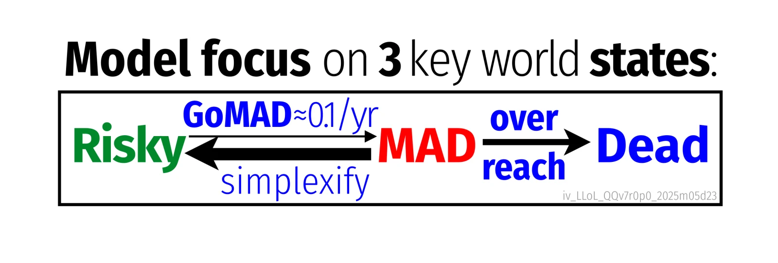
Figure 1: The whole model, in a box. The world leaves Risky for a MAD crisis at the crisis rate
(GoMAD, about 0.1 per year), leaves the MAD crisis back to Risky when it is simplified, and leaves
it forward to Dead by over-reach. That is all of it. The model code behind this diagram is
short enough to read over coffee and to run yourself (SIA-1), and it is shown as an invitation:
disagree with a number, change it, and see what comes out — or write a better model.#
((( The title’s “deep uncertainty” is not a hedge. It names the situation honestly: we cannot watch the true state of the system directly, so we price what we cannot see, from the traces it leaves. )))
4. Numbers That Count#
Feed the record’s rate into the model and it returns a distribution, not a point. These numbers are the basis for the decision in the next section — not the decision itself.
How this paper states its numbers, and why it costs itself something to do so
Every figure quoted in Sections 4 to 11 is stated as a bound that under-claims, not as a point estimate. Where the exact value is one in thirty-four, the text says worse than one in forty; where it is fifty-eight-fold, the text says more than fifty-fold. The rounding always runs against this paper’s own case, so that no claim in the ring can be defeated by a reader who recomputes it and finds the true figure smaller than advertised — it will be larger.
This is deliberate and it is borrowed. It is the rule a German commercial balance sheet has to obey: value cautiously, recognise foreseeable losses as soon as they are foreseeable, and recognise gains only once they are realised — so that the reader of the accounts is never surprised in the unfavourable direction (SIA-16). The appendices do the opposite, and must: they report exactly what the model returns, to the digit, because they are the audit trail and a rounded audit trail is no audit trail. So a reader comparing the two will find every appendix figure more favourable to this paper’s case than the ring’s claim about it — the danger a little larger, the remedy a little easier to justify. That gap is the discipline, not an inconsistency.
At the observed rate, the mean time to onset is about thirty years and half of all runs of world history are over within about twenty — twenty-one on the exact arithmetic, and even on the most sceptical published reading of the record, within about seventy. The chance that accidental nuclear winter begins in any given year is worse than one in forty; over a forty-year career, more than seventy percent. Across the full range the record can support — from the most sceptical published reading to the most pessimistic — the annual chance is never better than about one percent, and at the pessimistic end worse than one in fifteen. Forty simulated runs of world history agree with the exact arithmetic to within sampling noise (SIA-2, SIA-5), and the exact values behind every bound above are in Table 3 (SIA-5).
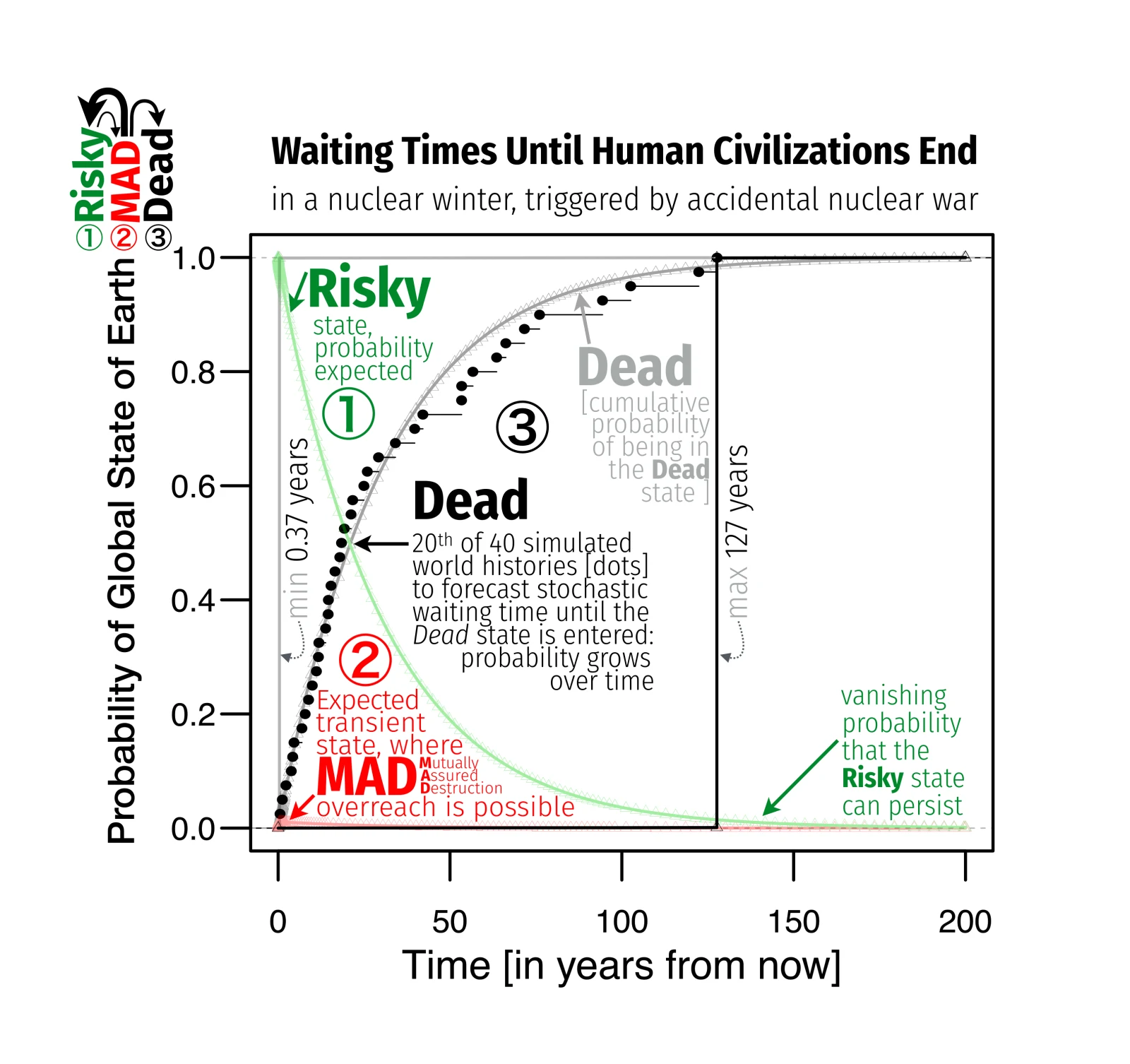
Figure 2: One world, read closely — the expected case, with every quantity labelled. Time runs left to right in years from now. The green curve is the probability the world is still merely Risky, falling as time passes; the red curve is the MAD crisis, a crisis in progress, which stays near the floor because crises are rare and short; the black dots and grey curve are Dead. Each dot is one simulated world history, placed at the year its own run arrived, and the grey line is the cumulative probability the arithmetic expects — the two agree. Read off the right-hand panel: 5 percent of runs are over within 2 years, half within 19, 95 percent within 103; the fastest run took 0.37 years and the slowest 127. That is the whole method in one picture. The next two figures do only two further things: change the crisis rate, and pool the runs. 40-run stochastic simulation (distribution shape); exact values in Table 3 (SIA-5).#
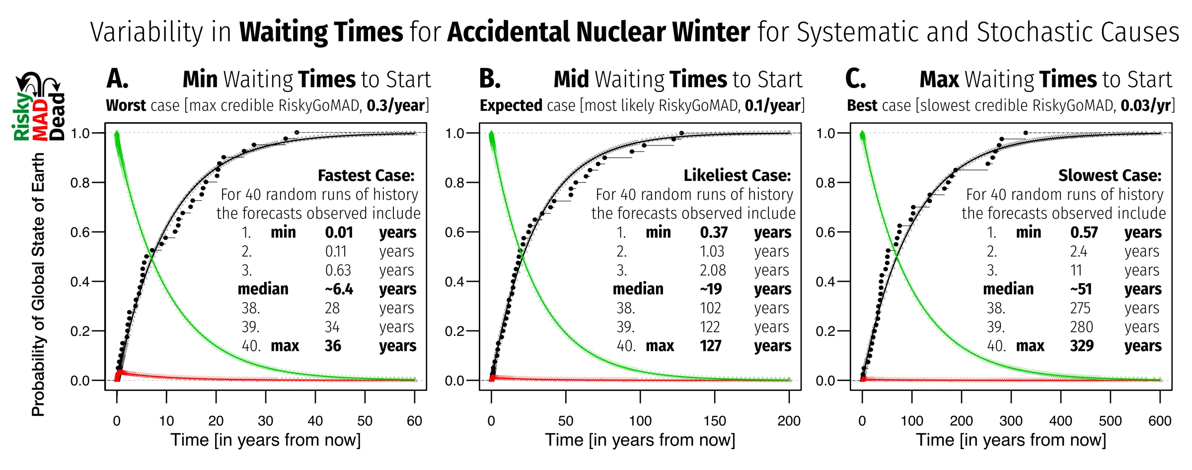
Figure 3: The same picture, in three worlds, worst first. A. the worst credible crisis rate (0.3/yr): median about 6.4 years, slowest run 36. B. the expected rate (0.1/yr): median about 19 years, slowest run 127. C. the best credible rate (0.03/yr): median about 51 years, slowest run 329. Note the x-axes: 60, 200 and 600 years. The argument holds equally whether the waiting time is four days or three centuries — which is the point of showing all three. 40-run stochastic simulation (distribution shape); exact values in Table 3 (SIA-5).#
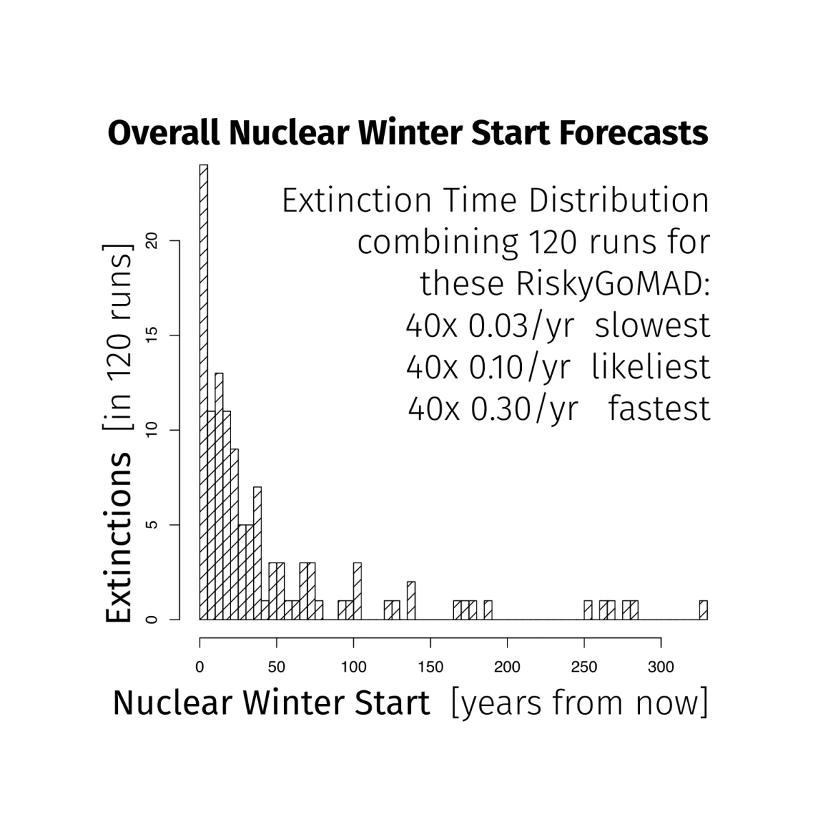
Figure 4: The same 120 runs pooled — the shape of the forecast. Most runs end early; a thin tail reaches three centuries. This is what a distribution with no way out looks like: not a deadline, but a schedule of chances. 120-run stochastic simulation, 40 runs at each of 0.03, 0.10 and 0.30 per year (distribution shape); exact values in Table 3 (SIA-5).#
One comparison makes the scale legible. Discounted by the share of humanity a nuclear winter kills, an individual’s annual chance of dying from accidental nuclear winter is more than fifty times the global road-death rate — counted the same way, death for death, year for year, person for person. ((( In plain terms: for most people alive today, this is a likelier way to die than a car crash. ))) This inequality is the paper’s one invariant claim. It holds in every scenario — even the most optimistic, which is the most sceptical published critic’s own rate, where it still stands at more than fifteen times the road-death baseline (SIA-9, SIA-10) — and it survives, threefold, when the most sceptical rate, the lowest published death toll, and the worst national road-death rate on record are imposed all at once (SIA-9). No single figure here is offered as invariant. The inequality is.
And because Dead is absorbing, the distribution has a long tail but no way out. Even a single year is not negligible: it is a revolver whose cylinder holds fewer than forty chambers and one round, held to the head of civilization, and fired once a year, every year. The most optimistic scenario widens the cylinder — to fewer than a hundred and twenty. It does not unload the gun. ((( This is what “stochastic certainty” means: not that it happens this year, but that, left unchanged, it happens — the dice turn up the six eventually. )))
5. Choice: Will We Survive Nothing?#
Proposed wording for LLoL’s approval — the ring’s centre (the decision call)
Section 5 is the latch of the whole ring; its voice is LLoL’s to set. It is written here in secular terms; the older sources that state the same choice with unusual clarity are set out, for readers who want them, in SIA-14. Calm register — surrender, not triumph; no self-nomination.
Everything before this section is the basis. What follows from it is not another number. It is a choice — and, stated in the right order, it is as old as the first community that had to decide whether to keep watch or not. In modern terms: am I my nuclear sibling’s keeper?
The clearest way to put it is to name the default first, because defaults are honest starting points. Death is not only what happens if we choose wrongly; death is what happens if we choose nothing at all. So the decision is between a death that arrives on its own and a life that has to be chosen to evade it.
0. Death by default. The threat from accidental nuclear winter gets ignored by most people most of the time — as it mostly has been for decades.
Imagine a highway with billions of lanes, all running forward. Only one or two will take you to the exit you actually want; the rest all lead to the same place. That is the shape of the choice — almost every lane is the broad road, and it takes deliberate effort to be in one of the few that is not.
The broad road runs on a single habit: blindly assuming blind leveraging. Cut the short-term corner, assume without looking that it is safe, and cut the next one — until the corners run out. It is the self-organizing pattern that emerges when everyone stays in their lane and does nothing — the fate of every system, work, or project that keeps cutting the short-term corner, and, as the Matheo Study Series shows, the pattern that ends in self-destruction. It asks nothing of anyone. To take it you need only do nothing — and it costs nothing today, which is exactly why it is the default.
But nothing is not the absence of a choice; it is a choice disguised as drift — and a shifting one. Nothing is never quite the same twice: it keeps changing shape, so that no one can quite name what was neglected, and no one can be blamed. The blindness is in the assuming — you keep taking the leverage and never look up to see where it is carrying you. The wheel keeps spinning. The watch is left to no one. The “not yet” becomes simply “now” — and by the time you glance in the rear mirror and see the exit you wanted, the road has already carried you past it. I have missed such an exit myself, and wrote down what I saw in the mirror Matheo-b19. Because no rule is broken and no one is keeping watch, no one sees it happen. That is what makes blindly assuming blind leveraging the most dangerous force there is: it ends the world while breaking none of its rules.
1. Life by choice. The narrow path — one of the few lanes that actually reaches the exit — asks the opposite discipline: zoning, investigating, organizing, navigating. Instead of assuming, you look: you map the ground, test what you find, put it in order, and steer by it. That deliberate work builds the information landscape that lets you see the exit while there is still time to take it. It is the self-correcting cycle this series calls for — the one that cannot be reached by drifting, only entered on purpose, at some cost, while the door is still open.
Stripped to its secular core, choosing it is choosing the open, unending search for truth — Real Quests for Real Answers: whoever goes on a real quest will find real answers, the continual and fearless sifting and winnowing by which alone the truth can be found — and choosing it out loud, in front of others, because a search that no one will publicly stand behind never gets funded, staffed, or believed. That public commitment is what turns a lone question into an institution: a ResearchCity, where the search is done full-time and in the open. And because a search whose fruits are hoarded in an ivory tower curdles back into the thing it replaced, the same choice carries a second half — a Jubilee-based cycle that returns those fruits, on a regular schedule, to everyone. Truth sought openly, housed in a ResearchCity, and shared by a Jubilee: that is the whole of “life by choice”, and it is also what lets rival powers keep competing without having to destroy one another. In the nuclear case its first concrete act is modest — that a qualified human, not a machine by default and not no one, be tasked to keep this particular watch, gentle kind reasonable, for everyone. It costs more today. It is the only road with a tomorrow on it.
That is the entire decision, and it is binary because the arithmetic is binary: either an absorbing state is reached, or the game is changed. There is no third road that quietly works out on its own.
((( “Will we survive nothing?” is meant literally. The thing most likely to end us is not a villain but a vacancy — the job no one is given, the risk that is, by definition, no one’s. )))
A personal statement (LLoL) — one voice, binding no one else
Imposing on no one, the author names his own answer — the only one he is entitled to name:
I have made up my mind to keep calling for Jubilee-based solutions — until the case is proven wrong, or I die, or a Jubilee-based reset is organized. If a better-worked path appears, I will follow it, after I audit its math. Until then, this one is mine. The choice above stays entirely yours.
Note
Where the older sources come in (→ SIA-14). Three of history’s clearest statements of exactly this gate-keeping choice — and the reason “life by choice” turns out to be the same thing as “keep searching for the truth, in the open, together, and share what you find” — come from Moses, Joshua, and Jesus. SIA-14 sets out the scriptures and maps each, line by line, to the secular terms used here. It is offered as depth, not premise: nothing in this section depends on it.
6. A Solution for the 10 Nuclear Kings#
A forecast delivered without a course of action gets filed and forgotten, so this paper carries its remedy. The current arrangement, Mutually Assured Destruction (MAD), has kept the peace for eighty years, and the model does not deny it. What the model adds is one word: metastable. MAD is a ball balanced on the rim of a bowl, not resting at its bottom — stable against small shocks, certain to fall given a large enough one. The arithmetic of Section 4 is the measure of how shallow the rim is.
The alternative this series derives is Mutually Assured Progress (MAP): change the game so that cooperation, not defection, is the rational move. A credible first-mover who acts at genuine, irreversible cost turns a stand-off in which each side is right to keep its arsenal into one in which each side is right to reduce, provided it can trust the others to. ((( The trick is not to ask anyone to trust blindly. It is to make one move so costly and so public that it cannot be a bluff — which is what lets the next player move too. )))
This is not hypothetical: the move has been made twice, and both times it worked. The first was B-59 in October 1962 — the decision Section 1 opens with, told in full in SIA-X7. On the only source there was no vote and no lone refusal: a captain who had ordered the nuclear torpedo readied consulted Vasili Arkhipov and the political officer and surfaced instead — into the enemy’s searchlights, unable to dive, at real cost, with no way of knowing he was right. In the late 1980s Mikhail Gorbachev made exactly this kind of concession: visible, costly, checkable, and made first. Each won a world war by making it never happen — and neither is commemorated for it. Both were Russians; and the Russian tradition even has a word for one who acts rightly while the world calls it folly — the yurodivy, the holy fool who says what power does not want to hear. At a moment when much of the world sees only a threat from that direction, the debt is worth naming plainly: the only two moves that have ever defused this danger were made from that side. This paper asks for a third.
Note
On the Arkhipov account, and why the argument does not stand on it. The dramatic version of the B-59 story is contested; the objection — Tertrais (2017) [Tertrais, 2017] — is set out where the story is told in full, in SIA-X7, and is not repeated here. For this section the point is narrower: the MAP first-mover claim rests at least as much on Gorbachev, whose concessions are uncontested, and no number anywhere in the paper moves if the Arkhipov account is read at its most sceptical.
The sovereigns who would have to permit the escape are addressed here as the ten Nuclear Kings — a deliberately ironic title, since ten cannot all be sovereign over one shared fate. ((( “King” here just means the holder of an unappealable decision. The ten are nine that hold weapons — the United States, Russia, China, North Korea, India, Pakistan, Israel, France, the United Kingdom — and one, Iran, whose intent to join is declared. The word “Nuclear” is never dropped. ))) A thousand years ago King Cnut had his throne carried to the sea and commanded the tide to halt — and the story is almost always told backwards. He staged it on purpose, in front of his courtiers, so that they could watch him fail, because they had been flattering him that all things obeyed him. The tide here is the table in Section 4. It does not negotiate, grants no exception for arsenal size, and holds no opinion about anyone’s sovereignty. Bowing to it early, in front of witnesses, is not defeat; it is the one move a king can make and still be remembered as wise.
Concretely, the ask is a window — an Earth in Escrow: a seven-to-fourteen-year peace in which the escape is actually built, while the arithmetic is checked by the people who hold the classified data that could settle it. The escape is a ResearchCity: an institution to do, full-time and in the open, the work of catching the thousand quiet ways a system fires by accident — work that no single discipline, and no lone hero, can hold. It is meant as a “Ministry of Nothing”: it takes on the threats that are nobody’s job so far — such as estimating how long we can expect to wait until an accidental nuclear war — works in the gaps between existing institutions, and hands what it finds to whoever is best placed to act. Before its seven scale-up stages comes a Stage 0, the preparation: one person’s model, checked by a small team and then by a pilot group of about 150 reviewers, while the world decides whether to give ResearchCity a mandate (ResearchCity: How to get there). It is one proposal; the forecast stands without it. And, following the oldest template for a warning of this shape, the paper does not nominate who should run it. Reading Pharaoh’s dream of coming famine, Joseph did not say make me the man; he said find a discerning one and set him over the land (SIA-14). The recommendation to the conveners is exactly that: find someone. What the window costs is priced in Section 9; the full mechanism, the game-theory, and the companion results are in SIA-13.
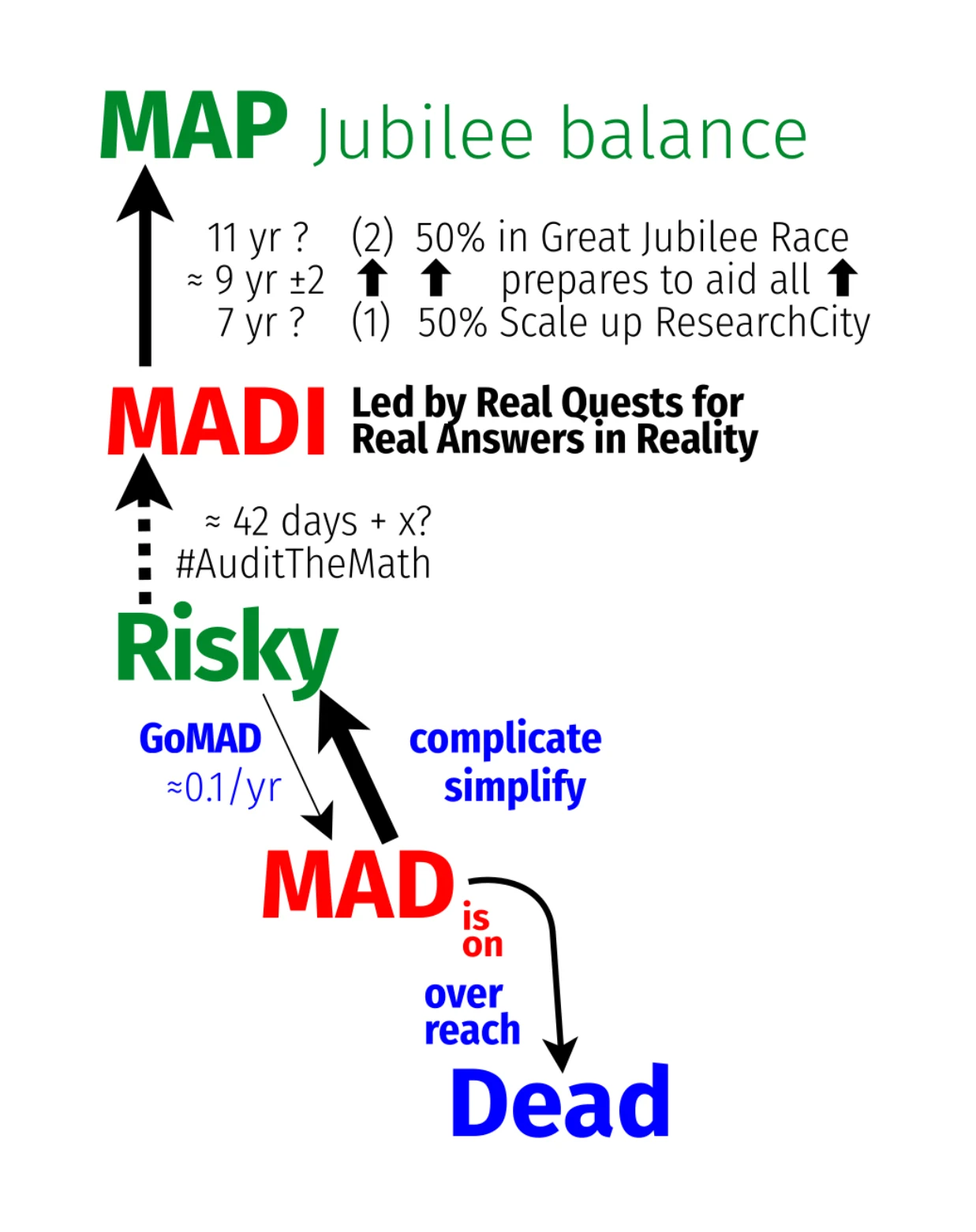
Figure 5: The escape drawn on the same model. Downward from Risky runs the path the forecast prices: into a MAD crisis, and by over-reach into Dead. Upward runs the alternative: MADI, a decision to be led by real quests for real answers in reality — reachable, on this sketch, in about forty-two days plus however long it takes to decide (the best case of ResearchCity’s Stage 0, whose last step is that global decision) — and from there, in two staged halves (scale up a ResearchCity, then run the Great Jubilee Race), to MAP and a Jubilee-based balance. The stage labels carry question marks because they are estimates, not promises: about five years to the first half; the whole escape takes seven to fourteen years, nine to eleven expected (Section 9, Table 8). The upward path has rate zero today because nothing has been built (SIA-1, SIA-13). #AuditTheMath#
7. Why Quiet Years Fool Us#
The obvious objection: if the risk is this high, why have eighty-one years passed without a nuclear war? The model’s answer is that eighty-one quiet years are exactly what it predicts most of the time — and are therefore weak evidence about the rate, not reassurance about it.
The reason is the shape of the process. Onset takes two steps — first a crisis must arise, then it must fail to stop — and a two-step process of this kind saturates: it behaves like a mechanism that can only work so fast, and that sits idle far more often than not. ((( This is the same maths biochemists use for enzymes, the Michaelis–Menten law: a catalyst spends most of its time waiting and only occasionally acts. Here the world spends about ninety-nine percent of its time merely “Risky” and about one percent in the lethal state. ))) A system that is dangerous one percent of the time produces long calm stretches as a matter of course — and then ends one. That is why the intuition “nothing has happened, so it cannot be that bad” is so durable and so unreliable, and why the same model that gives a median wait of twenty-one years also lets an occasional lucky run pass a century. SIA-7 explains why this mechanism is the right one; SIA-8 gives its numbers.
8. Why “Later” Isn’t an Option#
The most comfortable assumption in nuclear policy is that this can be handled later. Three things make delay not a neutral choice but a losing one.
There is no safe waiting period. Because the Dead state is reached with probability one given enough time, no run of quiet years lowers next year’s odds; every year, the wheel is spun again.
There is no stable middle. A system that is not actively correcting itself drifts, by default, toward its failure mode — and the drift is invisible from the inside, because the appearance of stability (“deterrence is working”) is the very thing that stops anyone from checking. Apparent calm is not evidence of safety; it is the symptom most easily mistaken for it.
The “we’ll learn as we go” hope reverses its own burden. Each near-miss has indeed taught a lesson — the hotline after Cuba, better warning after Able Archer. But to solve the problem, learning would have to drive the crisis rate to exactly zero, which no one claims; and the assurance that deterrence is safely managed comes, overwhelmingly, from the institutions whose reason for existing is to manage it. That is not an accusation — it is a statement about incentives, and it applies to this paper’s author with equal force.
((( These four traits together — time running out, no central authority able to act, the people who cause the problem also offering the cure, and a future discounted so steeply that “later” always wins — are the textbook definition of a super-wicked problem. Nuclear risk is a member of that named class, which is why its ordinary machinery of correction does not engage. )))
9. Cost of the Escape-Hatch#
A plan that names a timeline can be priced by the same model that produced the problem, and it should be. The whole escape — scaling the ResearchCity up through its seven stages (about five years), a switch from inward to outward, then about as long again helping everyone else make the transition — is estimated at nine to eleven years, counted from the end of Stage 0. It has hard limits at both ends: no less than seven years, because each stage has to reach functional completion, and no more than fourteen. The model says what such a window costs.
Window |
optimistic |
base |
pessimistic |
|---|---|---|---|
7 years |
6.6% |
20.4% |
49.0% |
9 years (mid case) |
8.5% |
25.5% |
58.1% |
11 years |
10.3% |
30.3% |
65.5% |
This is the honest price, and it is not reassuring. At the base rate a nine-year plan carries no better than a one-in-four chance of not finishing in time. That is not a reason to reject it; it is the figure any alternative must beat — and the alternative, doing nothing, costs seventy-three percent over a career (Section 4), with no escape at the end of it. ((( A treaty alone will not do it: nothing in a treaty sets the crisis rate to zero. What the escrow window buys is only the time to build the escape — but that time is the whole game. ))) The staging and its softest assumptions are in SIA-13.
Now the question that does not depend on any of it. Everything above rests on a hazard rate that nobody outside this paper has yet checked, and a reader who doubts it has, so far, no way through. So here is a second calculation built not to need it — because it asks the question backwards. Not how big is the danger, which is the part in dispute, but: how small may the prospect of success be before paying for the attempt is still worth it? The first question can only be settled by people with better data. The second can be settled at a desk, by anyone, in about a minute.
Four quantities, each per person and per year, and each open to attack. \(K\) is what it costs — the ResearchCity at roughly eight dollars a person a year (SIA-13). \(r\) is the annual risk, from Section 4: 0.029 at the base rate. \(E\) is what is at stake for one person if it happens. \(p\) is the chance the spending works — the unknown, and the thing to solve for. Paying is worth it once the expected benefit clears the cost, \(p\,r\,E > K\), which rearranges to a threshold:
((( The units are the fastest check there is. \(p\) is a bare number, \(r\) counts per year, \(E\) is in dollars — so both sides read dollars per person per year, and a reader who tests nothing else should test that. )))
Three things about this inequality run against the case it is used to make, and are stated before the numbers rather than after. The benefit is counted for one year only, though an escape that works keeps working and the whole future after it is credited at zero. The cost is counted every year, though a threat retired stays retired. And the calculation says whether a given outlay is worth making — not what outlay would be best, which would require knowing how the prospect of success grows with spending, and nobody knows that.
\(E\) is a value judgement, not a measurement. What an averted nuclear winter is worth to one person is where the reader’s own values enter, and no arithmetic can settle it. So the paper reports a band and hands over the dial rather than pretending to a figure it could defend.
Why the band spans two orders of magnitude, and why that is not vagueness. What a life is valued at differs enormously between countries — a wealthy state’s regulator and a poor one’s health ministry work with figures that can lie a hundredfold apart, and any single number would invite the objection that it is somebody else’s. The band is set wide on purpose, to span that international spread, so that the conclusion cannot be defeated by disagreeing about whose valuation to use: it holds at every point in it. ((( This works here for a reason particular to the hazard. Nuclear winter is global and no one can be excluded from it, so a single figure per person is meaningful in a way it would not be for a local risk — everyone is in the same boat, and the arithmetic assumes exactly that and nothing more. )))
What the stake \(E\) is measured against, since the convention matters. \(r\) is the chance that onset begins, so \(E\) is the value of averting the whole event to one person — and it therefore already carries the fact that a given person may live through it. Setting \(E\) at one regulatory life-value is not the same as assuming one death: it prices a person’s own mortality risk at roughly a third of that figure, which is the death fraction this paper takes from the nuclear-winter literature (SIA-9), and everything else — the survivors, their descendants, and the conditions both depend on — at the remainder. A reader who thinks that remainder too small should raise \(E\), which lowers the threshold.
What one person’s stake \(E\) is set to |
at the base rate, the required chance is no more than |
and if the danger is overstated a hundredfold, no more than |
|---|---|---|
min — $90,000, a deliberately harsh floor: a hundredth of the ceiling below |
1 in 300 |
35 percent |
mid — $900,000, a tenth of the ceiling below |
1 in 3,000 |
3.5 percent |
max — $9,000,000, just under the US Department of Transportation’s own guidance value of $9.1 million in 2012 dollars [U.S. Department of Transportation, 2021] |
1 in 30,000 |
0.35 percent |
((( Every entry is a ceiling, rounded against this paper: the exact values are 1 in 326, 3,263 and 32,628, and 30.6, 3.1 and 0.31 percent (SIA-15). A reader who redoes the arithmetic will find the requirement easier to meet than the table promises, never harder. Note that the ceiling itself rounds down from the regulator’s $9.1 million rather than up, so that no rounding anywhere in this table runs in this paper’s favour. )))
Two notes a careful reader will want, because this table’s arithmetic does not round the way the rest of the paper does. First, it uses the exact base hazard, 0.029, and not Section 4’s under-claiming floor of one in forty. That is deliberate and it is the same rule applied, not an exception to it: here the direction reverses, because a smaller hazard makes the required prospect of success larger, so under-claiming the danger would over-claim the ease. Using the floor would have pushed the right-hand column past its own ceilings — 35.6 percent against a stated 35, and so on down the column — which is precisely the kind of quiet convenience the rule exists to prevent, so it is reported rather than adopted. Second, the most sceptical published reading of the record is only about three times below the base rate, so its thresholds fall between the two columns and much nearer the left: about one in ten thousand, one in a thousand, and one in a hundred across the three stakes. The right-hand column discounts thirty times further than the most sceptical reading anyone has published.
The robustness is the point, and so is where it stops. Take the danger to be overstated by a factor of a hundred — a median wait not of twenty years but of two thousand, far beyond anything the record can bear — and at a mid-range stake the required prospect of success is still no more than three and a half percent. A reader does not have to accept Section 4 to reach Section 11; being wrong about the hazard by two orders of magnitude does not reverse the answer. But it does not hold at every corner, and the corner is named here rather than left to be found: insist on the harsh stake and the hundredfold discount together, and the requirement rises to as much as thirty-five percent, which is a real hurdle rather than a low one. The conclusion survives that corner; the word “effortless” does not. ((( Which is the ordinary shape of a robustness claim, honestly stated: it holds across a wide range and it has an edge, and a reader is owed the edge. )))
And the prospect of success is a chain, not a hunch. \(p\) is not one guess but a product of links — the money arrives, the check actually happens, it is competent, it is right, and somebody acts on what it finds. Four links at only one chance in five each still give better than one in six hundred and fifty, which clears the mid-range ceiling nearly five times over. That is a harder thing to dismiss than a single optimistic number, because each link can be argued about separately.
Caution makes this easier to justify, not harder — and that result is parameter-free. The table above prices the loss at its plain money value, which is not how anybody responsible for a catastrophe reasons: a loss that takes everything weighs more than its arithmetic sum, because there is no replacement and no second attempt. Scoring the outcome with any risk-averse valuation lowers the threshold. Not for some parameter choices — for every concave valuation there is, with the plain-money case as the exact boundary. The threshold in Table 10 is therefore a ceiling, not an estimate. The proof, the standard closed form, and a worked cross-check are in SIA-15; the calculation’s known limits are in SIA-16.
A last note on what is actually being asked for. Table 10 prices the programme. What Section 11 asks for is the far smaller thing: that somebody competent spend a few weeks checking whether the hazard rate is right. That decision is not the same one, and it is strictly easier — because its payoff arrives whichever way it comes out. A careful public demonstration that this paper is wrong would retire an urgent claim and redirect the effort it is consuming, which is a real gain that the arithmetic above counts as zero (SIA-16). ((( Which is why the request in Section 11 is not “agree with me”. It is “find out” — and finding out that the number is wrong is the better of the two outcomes. )))
10. There Are No Alternatives#
Set the two roads side by side one last time, because the choice is usually mis-stated as safe status quo versus risky change. It is not. The status quo is not safe: it is a stochastic certainty of death, on a schedule the model has now drawn. The transition is not certain: it is a finite, priced risk followed by a way out. A finite risk that ends is not the same kind of thing as an unbounded one that does not — and no amount of discomfort with the transition changes which of the two the arithmetic prefers. There is no third road, and not because this paper forbids one: an absorbing state admits exactly two futures — it is reached, or the game is changed before it is.
Ruin, not risk. The distinction the arithmetic is leaning on has a name: repeated exposure to any positive per-period chance of an absorbing loss is a ruin problem rather than a risk problem, and precaution under exposure of that shape is a standard result rather than a special plea for this case [Taleb et al., 2014].
The disagreement does not reach the decision. The most sceptical published reading of the record (Tertrais, 2017 [Tertrais, 2017]) and the most alarmed (SIA-X2) are separated by about a factor of ten in the crisis rate. That gap is real, and this paper does not pretend to close it. The arithmetic shows it need not be closed: across the whole interval the record can bear — from Tertrais’s corner to the pessimistic one — the decision is the same, because the car-crash inequality holds at every point (SIA-9) and the state stays absorbing at every point (SIA-4). To overturn the conclusion, an optimist cannot argue that the rate is low: a low rate, spun once a year without end, still reaches the absorbing state with probability one. The optimist would have to argue that the rate is exactly zero — and no one does. Tertrais himself grants that “even ‘virtually impossible’ does not mean zero.” A positive number, however small, together with an absorbing state, is the whole of the argument; the size of the number sets the schedule, not the outcome.
11. Call to Action#
Experts and officials move when there is public interest and — on the evidence of a year of letters that reached no one empowered to act — not much before. There is, at present, no channel: no procedure by which an existential-risk analysis reaches a desk that can act on it, and the procedures that do exist are built to discard exactly this kind of message (SIA-13). That is not a complaint; it is the reason the smallest action is the operative one, and why the call begins with everyone.
Step 0 — for everyone, and it is not “check the maths first”. The maths is a professional afternoon’s work for those equipped for it and an unfair burden for everyone else, so gating support on it would be absurd. The real question at Step 0 is a decision about trust: do you want this reviewed? Would you rather keep trusting an arrangement in which what gets measured is decided by who pays — the reason a number this simple went uncomputed for eighty years — or back people trying to do it in the open instead? If the latter, say so out loud: make some gentle, kind, reasonable, but unmistakable noise. It is, in the end, a wager on the unthinkable in insurance: nuclear war was ruled uninsurable because no one survives to pay a claim, so the only “policy” that can exist is to buy the risk down, by prevention — which is what a ResearchCity is for.
And the arithmetic makes that decision smaller than it looks. Nobody is asked to believe the forecast. Section 9 puts the question the other way round — how small may the prospect of success be before paying for the attempt is still worth it — and even with the danger itself discounted a hundredfold, the answer at a mid-range valuation of what is at stake is no more than three and a half percent. The request therefore hangs on the weak number rather than the strong one: it is enough to hold that the escape route is not ruled out. ((( Which is also the honest limit of what this author can ask for. He is not in a position to check his own work — years spent on something produce confidence about a person, not about the world, and the two can lie far apart (SIA-16). )))
Step 1 — experts: audit the maths and publish what you find. A refutation that retires a bad claim early is worth more than any number of agreements; every input is public and the method repeats in an afternoon.
Step 2 — those who can convene (the United Nations, Pope Leo XIV, and the ten themselves): put the waiting-time question on a table, and find someone to steward the escape. Under the game of Section 6, the first to move credibly, at cost, does not merely start a conversation — that move is the mechanism that shifts everyone else’s incentive.
Step 3 — everyone who can: help fund making the review transparent, and the ResearchCity, at roughly two cents a day — capped so no one can buy it, and half given away so no one can corner it.
The two requests, plainly. To whoever can convene: convene, and let the people with the classified data say whether the arithmetic is wrong — if it is, that is the best available outcome. To everyone else: check what you can, pass it on, and say what you find. Don’t believe it — #AuditTheMath. If the model is wrong, the fastest way to learn it is for someone to say so — and that is a better outcome than being right.
Supporting Information Appendices#
The SIAs hold all rigour and depth; the ring only states and points. SIA-1–14 follow the restructuring
proposal; SIA-15 and SIA-16 were added afterwards and carry the decision arithmetic behind Section 9
— the break-even threshold and the risk-aversion result (15), and everything that calculation does not
establish (16). The X-series (SIA-X1–X7) holds the standalone appendices: provenance and method (X1),
the rising crisis rate (X2), the field report on delivery (X3), the eighty-one anniversaries (X4), and
why numbers like this go unmeasured (X5) — all five carried over in the OOv2 → OOv3 port — plus
the draft-status and change record (X6) and the full B-59 account behind the paragraph Section 1 opens
with, together with what is contested in it (X7). The appendix numbering will be consolidated in a
single end-pass; the X prefix keeps the others stable meanwhile.
SIA-1 — The model itself#
RiskyMAD is a three-state continuous-time Markov chain, small enough to state in full and to solve exactly (SIA-4).
Risky — the current state: nuclear weapons exist and are deployed, but no exchange has occurred. The state is metastable — it appears stable yet carries a non-zero probability per unit time of leaving.
MAD crisis — a crisis in which nuclear exchange becomes imminent. The state is transient: it either escalates to Dead or de-escalates back to Risky. Mean crisis duration in the model is \(1/r_{M \rightarrow \text{out}} \approx 40\) days, consistent with historical crises (the Cuban Missile Crisis lasted thirteen).
Dead — accidental nuclear winter has begun. The state is absorbing: once entered, it cannot be left. It is named for the irreversible collapse of the civilization that produced the weapons, not because every human dies; limited exchanges that do not trigger a global winter are not modelled as “Dead” but as milestones toward normalizing one.
Four transitions connect them:
Risky |rarr| MAD crisis (
rMADcrisisStarts\(= r_{R \rightarrow M} = 0.10\)/yr) — a crisis brings the system to the nuclear brink.MAD crisis |rarr| Risky (
rMADcrisisCalms\(= r_{M \rightarrow R} = 6\)/yr) — the crisis de-escalates without exchange.MAD crisis |rarr| Dead (
rMADcrisisToWinter\(= r_{M \rightarrow D} = 3\)/yr) — the crisis escalates to exchange and accidental nuclear winter.Risky |rarr| LifeMAP (
rRiskyEscape\(= 0\)) — the escape to Mutually Assured Progress. Its rate is zero in the base model because no escape mechanism is currently active (Section 9, SIA-13).
The per-crisis death probability is the derived ratio \(p_{M \rightarrow D} = r_{M \rightarrow D}/r_{M \rightarrow \text{out}} = 3/9 = 1/3\); its structural justification and the calibration of the crisis rate are in SIA-6.
Figure 6: The three states and the three active transitions, repeated here from Section 3 beside the code they correspond to. The fourth transition, Risky → LifeMAP, is not drawn because its rate is zero: nothing has been built. Drawn in, it is Figure 5 (Section 6); as code, it is Figure 9 (SIA-13).#
The complete model code, as published on the SD1 poster, implemented in the Evolvix prototype compiler (MMv0r3p1-RC1) and run as an exact stochastic simulation by the Gillespie (1977) algorithm:
Evolvix Quest RiskyMADdead
(Question: "How many years until humanity self-destructs
            in a nuclear roulette accident?")

Simulate stochastically until 200 :["years"]

Initial Amount of Risky       = 1
Initial Amount of MAD         = 0
Initial Amount of Dead        = 0
Initial Amount of rMADcrisisStarts = 0.10
Initial Amount of rMADcrisisCalms = 6
Initial Amount of rMADcrisisToWinter = 3

Action 1 ( Risky ---[ Rate = 0.10 ]---> MAD     )
Action 2 ( MAD   ---[ Rate = 6    ]---> Risky   )
Action 3 ( MAD   ---[ Rate = 3    ]---> Dead    )
Action 4 ( Risky ---[ Rate = 0    ]---> LifeMAP )
This is the entire model. Implementing a Gillespie-dynamics continuous-time Markov chain in a general framework takes hundreds of lines; in Evolvix it fits on a poster, and anyone who can read the code can check the math. The compiler is available for download at Evolvix Prototype Compiler — Download and RiskyMAD Model Code.
Notation (BEST Names). Every quantity carries a Brief symbol for equations, an Explicit name as it appears in model code, a Summarizing phrase for prose, and a Technical column tying it to the cross-paper and enzymology identities (SIA-7). The convention is developed for semantic reproducibility across code-to-brain interfaces [Loewe et al., 2017]; a reader who never looks at an equation loses nothing by staying in the Summarizing column.
Reading the Brief symbols. They are built from the three state names, so nothing has to be memorised: R = Risky (now) → M = MAD crisis → D = Dead (winter has begun). Then \(r\) is a rate per year, \(p\) a probability, \(T\) a time in years, \(n\) a count and \(q\) a fraction — and the subscript says between which states, so \(r_{R \rightarrow M}\) is “the rate of going from Risky to a MAD crisis”. Two quantities are named in words rather than arrows (\(r_{\text{onset}}\), \(r_{\text{relax}}\)) because they are not transitions: they come out of solving the model rather than going into it. The scheme was adopted on 2026m09d08; the last column below gives the symbol used in drafts before that date. Table 0 lists the ten quantities the body uses, and agrees with SIA-1 name for name. The exhaustive treatment is in SIA-1: Table B indexes all twenty-six on one page, the glossary gives the full entry for each, Table B-old maps every pre-2026m09d08 symbol, and Table B-MM reads the same quantities as enzyme kinetics.
Brief |
Explicit (model code) |
Summarizing (used in prose) |
Technical — synonyms and cross-paper identities |
before 2026m09d08 |
|---|---|---|---|---|
\(r_{R \rightarrow M}\) |
|
the crisis rate |
How often the world enters a nuclear crisis, per year. Hellman’s \(\lambda_{IE}\) (initiating-event rate) is the nearest published relative; his \(\lambda_{CMTC}\) is not this quantity — it is his end-to-end failure rate, comparable instead to this paper’s onset hazard below (SIA-10). Michaelis–Menten substrate \(S\) (SIA-7). |
\(\lambda\) |
\(r_{M \rightarrow R}\) |
|
the de-escalation rate |
How fast a crisis resolves back to safety, per year. Two of the three OSCR modes (SIA-6). |
\(b\) |
\(r_{M \rightarrow D}\) |
|
the kill escalation rate |
How fast a crisis resolves into nuclear exchange, per year. One of the three OSCR modes. Michaelis–Menten \(V_{max}\) — you cannot die faster than this. |
\(c\) |
\(p_{M \rightarrow D}\) |
|
the per-crisis chance of nuclear winter |
The fraction of crises that go all the way. Michaelis–Menten commitment to catalysis; specificity constant \(k_{cat}/K_m\). Kennedy’s Cuban estimate (SIA-6) is a reading of this quantity, not of the crisis rate. Not separately identified from the crisis rate — see Matheo-b16-extra, section 14.1. |
\(p_{death}\) |
\(T_{R \rightarrow D}\) |
|
the waiting time |
Expected years from now until onset. First-passage mean to absorption from state Risky. Not a half-life and not a deadline (SIA-X2). |
\(T_R\) |
\(q_{\text{dead}}\) |
|
the death fraction |
Share of humanity that dies once nuclear winter begins. Not produced by this model; taken from the nuclear-winter literature (SIA-9). |
\(q\) |
\(r_{\text{onset}}\) |
|
the onset rate |
The slow rate at which the whole system reaches Dead, per year. This is the number comparable to Hellman’s “1 percent per year” and to Tertrais’s implied rate — not the crisis rate (SIA-4). |
\(r_1\) |
\(r_{\text{relax}}\) |
|
the relaxation rate |
The fast root of the same quadratic — not a disaster rate, and not the crisis clock either. It is the speed at which the hazard settles to the onset hazard, and it exceeds \(r_{M \rightarrow \text{out}}\) strictly whenever \(r_{M \rightarrow R} > 0\) (Matheo-b16-extra, section 7.3). |
\(r_2\) |
\(r_{M \rightarrow \text{out}}\) |
|
the crisis clock |
\(= r_{M \rightarrow R} + r_{M \rightarrow D}\), the total rate of leaving a MAD crisis by either arrow; its reciprocal is the mean crisis duration, ≈ 40 days. Michaelis–Menten \(K_m\). |
\(b+c\) |
\(T_{M \rightarrow D}\) |
|
the waiting time from inside a crisis |
First-passage mean to absorption from a MAD crisis, counting every later crisis if this one de-escalates. A bookkeeping quantity of the derivation (SIA-4). |
\(T_M\) |
The RiskyMAD model and what it assumes#
Three potential states our Risky world can be in#
Risky — weapons exist and are deployed; no exchange has occurred. This is where the world is now. It looks stable and is not: it carries a small probability per unit time of being left.
MAD crisis — a crisis under Mutually Assured Destruction in which death by accidental nuclear winter is merely one push of a button away, and the chance that someone pushes it is \(p_{M \rightarrow D}\) = 1/3 for the purposes of this paper. The 1962 Cuban Missile Crisis is the type case. Temporary: it resolves one way or the other, on average within about 40 days.
Two cautions. First, “MAD crisis”, never bare “MAD” — for two reasons rather than one. MAD alone keeps its usual meaning of Mutually Assured Destruction, the doctrine, which is permanent, while the model’s state is a crisis under that doctrine, which is not. And a bare MAD set beside Dead is one glance away from being read as the state it leads to, when the entire forecast is about the distance between them: Dead is what a MAD crisis produces when it is over-reached. This paper therefore writes “MAD crisis” (or “MAD crises”) for the state everywhere, spells the doctrine out in full where the doctrine is meant, and leaves the model name RiskyMAD, the code identifiers and the mathematical subscripts at their established spelling. Second, the 1/3 and the crisis rate are one calibration, not two. Fixing the chance at 1/3 is precisely what defines which historical near-disasters count as MAD crises at all, and so what
rMADcrisisStartsis counting. They trade off exactly, and The crisis rate and the escalation probability are not separately identified is the one place that works this out — every later passage that might tempt a reader to vary one while holding the other fixed points back to it.Dead — accidental nuclear winter has begun. Absorbing: once entered, never left. The name refers to the irreversible collapse of the civilization that built the weapons, not to the death of every human. The model deliberately does not resolve what happens below that line: total extinction, and a scattered remnant restarting from something close to a pre-agricultural baseline, are both simply Dead. Nothing in the forecast depends on telling them apart (What the death fraction counts, and what happens after two years).
Three arrows for transition rates between states of the world#
Transition |
Rate |
In words |
|---|---|---|
Risky → MAD crisis |
\(r_{R \rightarrow M}\) |
the world walks into a MAD crisis |
MAD crisis → Risky |
\(r_{M \rightarrow R}\) |
the MAD crisis de-escalates, and the world walks back out |
MAD crisis → Dead |
\(r_{M \rightarrow D}\) |
the MAD crisis escalates to exchange, and winter follows |
A fourth arrow, Risky → LifeMAP (the escape to Mutually Assured Progress), carries rate zero throughout this document, because nothing that would give it a positive rate has been built. Everything below is therefore a forecast of what happens if nothing changes, which is exactly what a forecast is for.
Base-case values, calibrated in b16 SIA-6 and taken as given here: \(r_{R \rightarrow M} = 0.10\)/yr, \(r_{M \rightarrow R} = 6\)/yr, \(r_{M \rightarrow D} = 3\)/yr.
The assumption ledger for the RiskyMAD model#
Stated once, in full, so that no assumption has to be discovered later by a reader who feels ambushed.
Assumption |
What it buys |
What it costs, and where that is repaid |
|---|---|---|
A1. Time runs continuously; the world is in exactly one of the three states at each instant. |
A model with three numbers instead of a history with infinitely many. |
Coarseness. A limited exchange that does not trigger a global winter is not “Dead” here; b16 treats such an event as a milestone toward normalising conditions that will eventually lead to accidental nuclear winter. |
A2. Each arrow fires at a constant rate — the chance of firing in the next instant does not depend on how long the world has already been in that state (memorylessness). |
The entire closed-form solution. |
The strongest assumption in the model. Repaid in 10. What survives without the exponential assumption: the mean waiting time does not need it. Only the shape of the distribution does, and therefore only the short-horizon figures. |
A3. The rates do not change over time. |
A single answer instead of a scenario family. |
Almost certainly false, and b16 SIA-X2 argues \(r_{R \rightarrow M}\) is rising. This makes the forecast conservative in the direction that matters: What none of this establishes shows onset stays certain when the rates vary, and rising \(r_{R \rightarrow M}\) shortens the wait. Also, that is why this analysis is incomplete with its respective min-max simulations for the most pessimistic-optimistic case. |
A4. Crises are independent of one another. |
Simple counting of repeat attempts. |
If crises cluster, the variance grows. The mean is untouched (10. What survives without the exponential assumption). |
A5. The three rates are correct. |
The specific numbers. |
This is the real exposure, and no derivation can reduce it. See 15. Parked, deliberately — and the rule for when to unpark it. Any single number will almost certainly be wrong, however, the likelihood that all numbers in the min-max intervall are also wrong is substantially smaller (and arguably near 0 if the intervall is well-chosen) |
BEST Names — what every symbol is called, and why#
Symbols are a user interface. A reader who must keep a lookup table in working memory has less memory left for the argument, and the argument is the point. The BEST Names convention [Loewe et al., 2017] gives every quantity four forms at once: a Brief symbol for equations, an Explicit name as it appears in human-readable model code, a Summarizing phrase for prose explaining the gist of what it does, and a Technical column tying it to the names other fields already use.
The rule followed here: a reader who never looks at an equation should lose nothing by reading only the Summarizing column.
Table B — the BEST Names index, every symbol on one page#
Read this first — three letters carry the whole scheme
Every symbol is built from the three state names, so nothing has to be memorised:
R = Risky (now) → M = MAD crisis → D = Dead (winter has begun)
Then \(r\) is a rate per year, \(p\) a probability (no units), \(T\) a time in years, \(n\) a count (no units), and \(q\) a fraction (no units) — and the subscript says between which states. Years are the unit throughout this paper; nothing depends on that choice. \(r_{R \rightarrow M}\) is “the rate of going from Risky to a MAD crisis”; \(T_{R \rightarrow D}\) is “the time from Risky to Dead”. Two quantities are not arrows, because they are not transitions — they emerge from solving the model — and they are named in words instead (\(r_{\text{onset}}\), \(r_{\text{relax}}\)). That difference is deliberate: the notation itself says which quantities to put in and which ones come out.
The Explicit names follow the companion code’s own two conventions:
camelCase for the three model parameters, which are what you set, and
snake_case for everything computed from them. Where an Explicit name is
proposed rather than already present in riskymad_exact.py, the entry in
Every symbol in full — the glossary says so; the name is given anyway, so that every quantity in this
paper can be referred to without a symbol.
The table below is exhaustive. Every symbol that appears anywhere in this paper is in it, including the ones a mathematician would consider too obvious to list — the discriminant, the sum of all rates, and the two local proof variables of The one fact everything rests on. Nothing is left for a reader to infer.
Brief |
Explicit |
Summarizing |
|---|---|---|
Put in — the three arrows of the model |
||
\(r_{R \rightarrow M}\) |
|
the crisis rate — how often the world walks into a MAD crisis. 0.1/yr, one per 10 years. |
\(r_{M \rightarrow R}\) |
|
the de-escalation rate — how fast a MAD crisis walks back to Risky safety. 6/yr. |
\(r_{M \rightarrow D}\) |
|
the kill escalation rate — how fast a MAD crisis explodes into nuclear winter. 3/yr, the committed step. |
Put in — one number from outside the model |
||
\(q_{\text{dead}}\) |
|
the death fraction — share of humanity dead within ≈ 2 yr of onset, all causes. b16 uses 0.3; scenario-matched is 0.63. |
Comes out — rates |
||
\(r_{M \rightarrow \text{out}}\) |
|
the crisis clock — how fast a crisis resolves, either way. 9/yr; 1/it is the mean crisis duration, ≈ 40 days. |
\(r_{\text{onset}}\) |
|
the onset rate — the disaster rate: 0.0331/yr = 3.3 %/yr, the level risk settles at. Compare published “X % per year”. |
\(r_{\text{relax}}\) |
|
the relaxation rate — not a disaster rate: the speed risk settles at \(r_{\text{onset}}\). 9.067/yr; 1/it ≈ 40 days. |
\(r_{\text{flux}}\) |
|
the flux of worlds — onsets per world-year, 0.0330/yr. What a simulation measures: an ensemble property, not a hazard. |
\(r_{\text{all}}\) |
|
the sum of every rate — 0.1 + 6 + 3 = 9.1/yr. Vieta: \(r_{\text{onset}} + r_{\text{relax}} = r_{\text{all}}\) checks both roots. |
Comes out — probabilities, counts, densities |
||
\(p_{M \rightarrow D}\) |
|
the per-crisis chance of nuclear winter — of all crises begun, the share reaching Dead. 1/3. Not a personal risk. |
\(n_{MAD}\) |
|
the number of MAD crises passed through before one ends it. 3 on average — this is \(1/p_{M \rightarrow D}\). |
\(p_{\text{winter}}(t)\) |
|
the density of the waiting time, in 1/yr — not a probability: only its area over a stretch of years is one. |
Comes out — times |
||
\(T_{R \rightarrow D}\) |
|
the waiting time — years until onset of nuclear winter. Mean 30.3 yr, median ≈ 21 yr; a distribution, not a date. |
\(T_{M \rightarrow D}\) |
|
the waiting time from inside a crisis — counting every later crisis too, not just this one. 20.3 yr — years, not days. |
Local proof devices, used once |
||
\(\Delta\) |
|
the discriminant — \(r_{\text{all}}^{2} - 4\, r_{R \rightarrow M}\, r_{M \rightarrow D}\). Its only job: to show both rates are always real. |
\(C_{M \rightarrow R}\) |
|
the calming clock — the random time until this crisis would de-escalate, if nothing else happened first. A time, in years. |
\(C_{M \rightarrow D}\) |
|
the winter clock — the random time until this crisis would reach Dead. Whichever clock rings first decides. |
Reported quantities — computed from the above, and quoted in the text |
||
\(r_{R \rightarrow L}\) |
|
the exodus rate — how fast the world sets out for Mutually Assured Progress. Zero so far, and not a constant of nature: it is what deliberate preparation raises, and it has to outrun the crisis rate to matter. |
\(r_{\text{winter}}(t)\) |
|
the hazard now — given the world is still here at
\(t\), the chance per year of onset. Starts at exactly
zero and climbs to |
\(P(T \leq t)\) |
|
the chance winter has begun by \(t\). 2.90 % for the coming year, against 3.25 % if the present calm is ignored. |
\(P(T > t)\) |
|
the chance it has not — the survival curve. \(= 1 -\)
|
\(T^{\text{med}}\) |
|
the median wait — 21.1 yr, well below the mean of 30.3. Half of all runs are over by then. |
\(\text{SD}(T)\) |
|
the spread of the wait — the standard deviation, from \(1/r^2_{\text{settled}} + 1/r^2_{\text{warm}}\). The distribution runs from days to centuries. |
\(r_{\text{naive}}\) |
|
the naive product — |
\(r_{\text{road}}\) |
|
the road-death baseline — 1.49e-4 per person-year, global. Put in, from outside. The car-crash comparison divides by this. |
\(n_{\text{road}}\) |
|
how much likelier than a car crash — 58x at the base
case. = |
\(S/K_m\) |
|
the saturation — 0.011, i.e. ninety times below half-saturation. How far the system sits into the first-order regime (SIA-8). |
Three things have been taken out of this table on purpose, each into its own place below, so that the index stays one page and each fact is stated once: the full explanation of every symbol (Every symbol in full — the glossary), the map to the symbols this document used before 2026m09d08 (Table B-old — the symbols this document used before 2026m09d08), and the enzyme-kinetics mapping (Table B-MM — the same quantities, read as enzyme kinetics).
Every symbol in full — the glossary#
The index above answers “what is this?” in two lines. This glossary answers “why is
it called that, what else is it known as, and what must I not confuse it with?” — and
it is a Sphinx glossary rather than a table for one reason: every entry is a :term:
target, so any later section of this paper, and any other paper in the series, can write
:term:`rWinterSettled` and link straight here. On the website a reader gets the definition
as a hover tooltip without leaving the page. In print it sets as the definition list it
already is, so nothing is lost.
Each entry is keyed on its Explicit name, which is why every quantity needed one. Where that name is a proposal rather than an identifier already in the companion code, the entry says (proposed) and names what the code does instead.
Six of these quantities carry a second complete set of names, because the model is
identical to Michaelis–Menten enzyme kinetics rather than merely analogous to it.
Those names are gathered once in Table B-MM — the same quantities, read as enzyme kinetics rather than repeated entry by
entry: rMADcrisisStarts, rMADcrisisCalms, rMADcrisisToWinter,
rMADcrisisEnds, pMADcrisisToWinter and rWinterPerWorldYear.
- rMADcrisisStarts#
\(r_{R \rightarrow M}\) — the crisis rate
Explicit: declared in the Evolvix model and used under the same name in the Python code.
how often a Risky world walks into a MAD crisis, per year
Technical: Poisson arrival rate. Hellman’s \(\lambda_{IE}\) is the nearest published relative. Textbook generator entry \(q_{RM}\).
- rMADcrisisCalms#
\(r_{M \rightarrow R}\) — the de-escalation rate
Explicit: declared in the Evolvix model and used under the same name in the Python code.
how fast a MAD crisis walks back to Risky safety, per year
Technical: Queueing service rate. Textbook \(q_{MR}\).
- rMADcrisisToWinter#
\(r_{M \rightarrow D}\) — the kill escalation rate
Explicit: declared in the Evolvix model and used under the same name in the Python code.
how fast a MAD crisis explodes into accidental nuclear winter, per year, if this MAD crisis was to actually last for a year.
Technical: Textbook \(q_{MD}\).
- rMADcrisisEnds#
\(r_{M \rightarrow \text{out}}\) — the crisis clock
Explicit: proposed here. The Python code writes the sum
rMADcrisisCalms + rMADcrisisToWinterinline rather than naming it.how fast a crisis resolves, either way (by mending or killing). Its reciprocal is the mean crisis duration, ≈ 40 days.
Technical: \(= r_{M \rightarrow R} + r_{M \rightarrow D}\), the total rate of leaving a MAD crisis by any arrow.
- pMADcrisisToWinter#
\(p_{M \rightarrow D}\) — the per-crisis chance of nuclear winter
Explicit: a named variable of the Python code; computed, not set.
of all the crises the world enters, the share that go all the way to Dead instead of back to Risky. Base case: 1/3. This number and the crisis rate are not separately identified: fixing it at 1/3 is what defines which near-disasters count as “Cuban-Missile-Crisis type” and are therefore counted by
rMADcrisisStarts. If the true per-crisis chance is higher than 1/3, the same forecast follows from a correspondingly higher effectiverMADcrisisStarts, and vice versa. Neither is known separately; what the study assumes is that their product lies between the bounds discussed in the text. Section 14.1 makes this exact.Warning
This is not anybody’s personal risk. “1/3” is a conditional about crises — given a crisis has begun, the share that run all the way. An individual’s annual chance of dying is a different quantity by two orders of magnitude: \(P(T_{R \rightarrow D} \leq 1) \times q_{\text{dead}} = 0.029 \times 0.3 \approx\) 0.9 % per year. Any reader who reads “1 in 3” as a personal odds has been misled by the notation, which is why \(p_{death}\) was retired as a name.
Technical: Computed by
p_end(). Same arrow as \(r_{M \rightarrow D}\), but a probability rather than a rate — which is why the defining identity \(p_{M \rightarrow D} = r_{M \rightarrow D}/r_{M \rightarrow \text{out}}\) can be read straight off the notation: the share of the leaving-rate that goes to D. Kennedy’s Cuban estimate is a reading of this, not of the crisis rate.- tUntilWinter#
\(T_{R \rightarrow D}\) — the waiting time
Explicit: a named variable of the Python code; computed, not set.
years from now (world is Risky) until onset of accidental nuclear winter (world is Dead after taking the wrong turn in a MAD crisis). A random quantity following a distribution, not a fixed date.
Technical: Computed by
mean_wait(). First-passage time to absorption from Risky. Not a half-life, not a deadline.- tUntilWinterFromCrisis#
\(T_{M \rightarrow D}\) — the waiting time from inside a crisis
Explicit: proposed here. It appears only inside the derivation, so neither code names it.
years from the start of some crisis until Dead, counting everything that follows if this crisis de-escalates: the return to Risky, the wait for the next crisis, and every later crisis until one of them ends it. Base case 20.3 years — note years, not the 40 days a single crisis lasts.
Technical: First-passage time to absorption from a MAD crisis. A bookkeeping quantity; it appears only inside the derivation. One symbol is enough, because the duration of the final crisis is not a separate unknown: by Fact 3 a crisis lasts \(1/r_{M \rightarrow \text{out}}\) ≈ 40 days on average whether or not it is the one that escalates. Check: \(1/r_{R \rightarrow M} + T_{M \rightarrow D} = 10 + 20.33 = 30.33 = T_{R \rightarrow D}\). ✓
- rWinterSettled#
\(r_{\text{onset}}\) — the onset rate
Explicit: a named variable of the Python code; it is computed, not set, so it has no place in the Evolvix model.
the composite rate, per year, of transitioning all the way from Risky through a MAD crisis to Dead. This is the disaster rate, and the one number here comparable to published estimates of “X percent per year” for nuclear war. Base case 0.0331/yr, that is 3.3 % per year. It is the level the risk settles at once the first months are past — not a rate that applies from day one (The hazard rises; it does not start at its final value).
Technical: Computed as the first value returned by
decay_rates(). Smaller root of the characteristic quadratic; the decay rate of the quasi-stationary distribution; the asymptotic hazard. It is an equilibrium rate in every sense that can apply to an absorbing chain. Strictly the chain has no equilibrium, since all probability drains into Dead (only 0.13 % of worlds survive 200 years); what it settles into is the quasi-stationary state — an equilibrium among the survivors, who divide 98.9 % Risky / 1.1 % in a MAD crisis. But that state has the defining property one would want: started from it, the waiting time is exactly exponential at rate \(r_{\text{onset}}\), with no correction term at any horizon (Which question is being asked — and what “we are not in a crisis today” is worth, checked to machine precision). It is not named \(r_{R \rightarrow D}\), because R → D is not a transition of the model: there is no direct arrow, only the composite journey through M. Bounded exactly by \(1/T_{R \rightarrow D} < r_{\text{onset}} < r_{R \rightarrow M}\, p_{M \rightarrow D}\) (Why the smaller root is the onset rate).- rRiskWarmsUp#
\(r_{\text{relax}}\) — the relaxation rate
Explicit: a named variable of the Python code; computed, not set.
not a disaster rate at all, and not a rival to \(r_{\text{onset}}\). The two are different kinds of quantity: \(r_{\text{onset}}\) is the level the risk settles at; \(r_{\text{relax}}\) is the speed at which it settles there, and its reciprocal, ≈ 40 days, is the relaxation time. Why there is anything to settle: the forecast is made knowing the world is in Risky today and not already in a crisis, so onset cannot happen immediately — a crisis must first arrive and then run its course. The risk therefore starts at exactly zero and climbs to \(r_{\text{onset}}\) within a few months (The hazard rises; it does not start at its final value and The shifted-exponential picture, and where the shortcut fails and Which question is being asked — and what “we are not in a crisis today” is worth). This is what that knowledge is worth: 2.90 % rather than 3.25 % for the coming year (Which question is being asked — and what “we are not in a crisis today” is worth).
Technical: Computed as the second value returned by
decay_rates(). Larger root of the same quadratic. Standard usage in kinetics and in Markov-chain theory calls \(1/(r_{\text{relax}} - r_{\text{onset}})\) the relaxation time; here the two differ by 0.37 % (40.43 d against 40.28 d), so the distinction never matters numerically but is stated to keep the identification honest. It is likewise close to, but not equal to, the crisis clock: \(r_{\text{relax}} = 9.067\)/yr against \(r_{M \rightarrow \text{out}} = 9.000\)/yr, larger by 0.74 %, and Why the smaller root is the onset rate proves that inequality is strict whenever \(r_{M \rightarrow R} > 0\). Section 7.3 explains why the two exponentials of the closed form are not the two physical stages.- nMADcrisesUntilWinter#
\(n_{MAD}\) — the number of MAD crises passed through before one ends it. 3 on average
Explicit: proposed here for the quantity; the Python code names only the function that returns it.
the number of MAD crises the world passes through before one of them reaches Dead — on average 3
Technical: Computed by
excursions(). Geometric random variable with success probability \(p_{M \rightarrow D}\). This is the factor that answers the “loop objection” (Reading the formula).- qHumansDead#
\(q_{\text{dead}}\) — the death fraction
Explicit: a named constant of the Python code. It is not in the Evolvix model, which does not need it: nothing in the simulation depends on it.
the share of humanity that dies within about two years of onset, from all causes taken together: the blast and fire, and then the famine and supply-chain collapse that follow, which dominate the total. It is not deaths in the strikes alone.
Technical: Not produced by this model. b16 SIA-9 takes it from Xia et al. (2022), whose figures are deaths by the end of year 2: a small regional exchange (~100 warheads, 5 Tg soot) gives about 2 billion (\(q \approx 0.25\)); a full US–Russia exchange (150 Tg) gives over 5 billion (\(q \approx 0.63\)). b16 uses 0.3, which is therefore conservative twice over — it takes the figure for the smallest exchange modelled, and it stops counting at two years while the climate disruption runs for a decade or more. Section 14.2 works through what the two-year horizon does and does not include; the scenario-matched value is 0.63, which would roughly double every multiplier b16 reports.
- rWinterPerWorldYear#
\(r_{\text{flux}}\) — the flux of worlds
Explicit: proposed here for the quantity; the Python code names only the function that returns it.
onsets per world-year, 0.0330/yr. This is what a simulation measures directly: run 40 world histories, add up their waiting times, and divide 40 by that total. It is a property of the ensemble, not of any world in it — a single world has exactly one onset, ever, on one date, and never experiences “0.033 onsets per year”. Distinct from \(r_{\text{onset}}\) in kind as well as value (0.0331/yr, 0.36 % apart): \(r_{\text{onset}}\) is a hazard — instantaneous, conditional on having survived so far — whereas \(r_{\text{flux}}\) is an unconditional average over the whole run. Quote \(r_{\text{onset}}\) against published “X percent per year” figures; quote \(r_{\text{flux}}\) when reporting what an ensemble of runs produced.
Technical: computed by
mm_velocity(). It is an ensemble average, not a hazard: onsets divided by world-years lived, which is what running many worlds and dividing measures.- rAllRatesAdded#
\(r_{\text{all}}\) — the sum of every rate
Explicit: a named variable of the Python code (
crosschecks.py; the localtotalinsidedecay_rates()).\(r_{R \rightarrow M} + r_{M \rightarrow R} + r_{M \rightarrow D}\) = 9.1/yr. It is a rate like any other and is written as one, rather than as a bare Greek abbreviation, so that an equation containing it can be looked up here. It grows automatically if the model grows: a Risky → LifeMAP escape arrow would enter this sum too.
Technical: Minus the trace of the transient generator. Appears in both Vieta relations: \(r_{\text{onset}} + r_{\text{relax}} = r_{\text{all}}\), which is the quickest check that the two roots were solved correctly. py``.
- dWinterPerYear#
\(p_{\text{winter}}(t)\) — the density of the waiting time, in 1/yr
Explicit: proposed here for the quantity; the Python code names only the function that evaluates it.
how much of the probability of onset falls in each year. Not a probability itself: it has units of 1/yr, and only its area over a stretch of years is a probability. It appears once, as the numerator of the hazard in section 7.2.
Technical: Evaluated by
pdf(). Probability density function of the waiting time. Lower case on purpose: \(P(\cdot)\) in these same equations is a probability, and a density is not one — the case carries the type. Named for the event rather than the arrow (winter, not \(T_{R \rightarrow D}\)) because a nested arrow subscript is unreadable at this size, and because accidental nuclear winter is what the whole paper is about.- underTheRoot#
\(\Delta\) — the discriminant
Explicit: a named local of the Python code, inside
decay_rates().the quantity under the square root when the two rates are solved for. Its only job is to show that the two rates are always real numbers rather than an oscillation, for any positive rates whatever (b16-extra section 6.5).
Technical: \(\Delta = r_{\text{all}}^{2} - 4\, r_{R \rightarrow M}\, r_{M \rightarrow D}\). Renamed from \(D\) in round four, because \(D\) is the state Dead in the arrow scheme and the two would otherwise appear in the same equations.
- tClockToCalm#
- tClockToWinter#
\(C_{M \rightarrow R}\), \(C_{M \rightarrow D}\) — the two clocks
Explicit: proposed here. A proof device: neither code has a counterpart.
a local proof device, used once and not needed afterwards. Picture each arrow as carrying its own alarm clock set to a random time; the MAD crisis ends when the first clock rings, and which clock rings decides whether the world walks back to Risky or arrives at Dead. Listed here so that a reader who meets these symbols in The one fact everything rests on is not left wondering why they were introduced at all.
Technical: Independent exponential random variables with rates \(r_{M \rightarrow R}\) and \(r_{M \rightarrow D}\). Conventionally written \(X\) in probability texts, where the letter carries no meaning; the clock reading is the same mathematics with an interpretation attached.
Table B-old — the symbols this document used before 2026m09d08#
This table exists to be deletable. It carries the whole of the old-paper tracking that was previously repeated inside twelve separate entries of the names table, and nothing else depends on it. Once every draft, llog and figure that used the old symbols has been migrated, this section can be cut in one edit and no other part of the paper changes.
Until then it is worth keeping visible rather than banishing to the repository. A reader holding a printout of an earlier draft, or a referee who saw a version before 2026m09d08, needs exactly this map and needs it in the paper rather than in a commit history. The third column is the separate question of what b16 itself calls each quantity, which is not a rename at all and does not go away when this table does.
before 2026m09d08 |
now (Brief) |
Explicit, before |
Explicit, now |
in b16 itself |
|---|---|---|---|---|
\(\lambda\) |
\(r_{R \rightarrow M}\) |
|
|
\(\lambda\) |
\(\mu\) |
\(r_{M \rightarrow R}\) |
|
|
\(b\) |
\(\kappa\) |
\(r_{M \rightarrow D}\) |
|
|
\(c\) |
\(\mu + \kappa\) |
\(r_{M \rightarrow \text{out}}\) |
— (new here) |
|
\(b+c\) |
\(p_{\text{end}}\) |
\(p_{M \rightarrow D}\) |
|
|
\(p_{death}\) |
\(W\) |
\(T_{R \rightarrow D}\) |
|
|
\(T_R\) |
\(W_{\text{crisis}}\) |
\(T_{M \rightarrow D}\) |
|
|
\(T_M\) |
\(r_{\text{slow}}\) |
\(r_{\text{onset}}\) |
|
|
\(r_1\) |
\(r_{\text{fast}}\) |
\(r_{\text{relax}}\) |
|
|
\(r_2\) |
\(n_{\text{tries}}\) |
\(n_{MAD}\) |
|
|
— (implicit) |
— (unchanged) |
\(q_{\text{dead}}\) |
|
|
\(q\) |
— (unchanged) |
\(r_{\text{flux}}\) |
|
|
\(v\) |
\(\Sigma\) |
\(r_{\text{all}}\) |
|
|
\(\lambda + b + c\) |
— (unchanged) |
\(p_{\text{winter}}(t)\) |
|
|
— (not in b16) |
— (unchanged) |
\(\Delta\) |
|
|
— (not in b16) |
\(C_\mu, C_\kappa\) |
\(C_{M \rightarrow R}\), \(C_{M \rightarrow D}\) |
— (new here) |
|
— (not in b16) |
Twelve of the sixteen changed. The four that did not — \(q_{\text{dead}}\), \(r_{\text{flux}}\), \(p_{\text{winter}}(t)\) and \(\Delta\) — are listed anyway so that the table can be checked for completeness against the index without holding anything in memory.
Table B-MM — the same quantities, read as enzyme kinetics#
Section 9 shows that this model is not analogous to Michaelis–Menten kinetics but identical to it. That makes the enzymology names a second complete set of names for the same quantities — which is why they are gathered here rather than scattered one clause at a time through the glossary.
This table is staged here and belongs in b16-extra section 9. It is a superset of Table F: it adds the two names Table F omits (\(k_{on}[S]\) and \(k_{off}\)) and the Explicit column. When it moves, it should replace Table F rather than sit beside it — see the note there.
Enzyme kinetics |
RiskyMAD (Brief) |
Explicit |
base value |
what it says here |
|---|---|---|---|---|
\(k_{on}[S]\) |
\(r_{R \rightarrow M}\) |
|
0.1 /yr |
Enzymology \(k_{on}[S]\). Michaelis–Menten substrate \(S\). |
\(k_{off}\) |
\(r_{M \rightarrow R}\) |
|
6 /yr |
Enzymology \(k_{off}\). |
\(k_{cat}\), \(V_{max}\) |
\(r_{M \rightarrow D}\) |
|
3 /yr |
Enzymology \(k_{cat}\), the committed step. Michaelis–Menten \(V_{max}\): you cannot destroy the world faster than this. |
\(K_m\) |
\(r_{M \rightarrow \text{out}}\) |
|
9 /yr |
Michaelis–Menten \(K_m\). |
\(k_{cat}/K_m\) |
\(p_{M \rightarrow D}\) |
|
1/3 |
Enzymology: commitment to catalysis; specificity constant \(k_{cat}/K_m\). |
\(v\) |
\(r_{\text{flux}}\) |
|
0.0330 /yr |
Michaelis–Menten reaction velocity \(v\) (9. Michaelis–Menten, derived rather than asserted), which is the same quantity read as a turnover: an enzyme processes substrate repeatedly, so for enzymes the flux is what one actually observes, and the ensemble is the molecules in the tube. Here the “tube” is a hypothetical population of worlds — which is exactly why the enzymology symbol \(v\) is kept only inside section 9, where that reading is being made on purpose. |
The mapping is exact at every value of \(r_{R \rightarrow M}\), not only in a limit; b16-extra section 9 does the substitution line by line and checks the defining half-saturation property. What the enzymology buys is not decoration: it is the reason the crisis rate can be counted from the near-disaster records rather than derived from a mechanism nobody can model — the same move that makes Michaelis–Menten useful for enzymes.
SIA-2 — LLoL’s SD1 analysis (the original approach)#
The first analysis of this model was LLoL’s, on the single-page SD1 poster (2024–2025, no AI). It ran world history forward as a stochastic simulation and read the waiting time off each run — the right instrument for the shape of the distribution (medians, long tails, the century-long quiet stretches on which the Michaelis–Menten reading of SIA-7 rests).
Method. Forty independent runs per scenario, generated with the Evolvix prototype compiler (download), which implements the stochastic simulation algorithm exactly (Gillespie, 1977; Ehlert & Loewe, 2014, “Lazy Updating,” J Chem Phys 141(20): 204109). Each run produces one random waiting time until accidental nuclear winter. Three scenarios span the crisis rate from optimistic (0.03/yr) through base (0.10/yr) to pessimistic (0.30/yr).
Figure 7: The base case, annotated — repeated here from Section 4 beside the method it illustrates. 1 (green) is the probability the world is still merely Risky, falling as time passes. 2 (red) is the thin sliver of probability sitting in a MAD crisis at any moment — about one percent of the time (SIA-8), which is why long quiet stretches are ordinary here (SIA-7). 3 is Dead: the grey line is the expected cumulative probability of having arrived there, and each black dot is one of forty simulated world histories plotted at the year its own run arrived. The forty runs and the expected curve agree. The fastest run took 0.37 years, the slowest 127. All three scenarios are compared in Figure 3. 40-run stochastic simulation (distribution shape); exact values in Table 3 (SIA-5). Source: SD1.#
What the runs showed. A median near 19 years at the base rate, with roughly one run in forty reaching catastrophe inside the first year, robust across death-probability scenarios (SIA-3 gives the summary table).
A limit of the instrument, stated plainly. Forty runs cannot resolve a 3-percent annual probability: the standard error on such an estimate at \(n = 40\) is about 2.5 percent, nearly the estimate itself. The simulations are the right tool for the distribution’s shape and the wrong tool for the one-year number; that number is supplied exactly by the arithmetic of SIA-4, and the two agree (SIA-5). No re-run would change this.
SIA-3 — LLoL’s summary statistics table (SD1)#
The forty-run simulation of SIA-2, tabulated. Kept as its own citeable unit, distinct from SIA-2’s method and from the exact arithmetic of SIA-5.
Scenario |
crisis rate |
median |
mean |
fastest run |
slowest run |
What the runs show |
|---|---|---|---|---|---|---|
Optimistic |
0.03/yr |
~51 yr |
~96 yr |
0.57 yr |
329 yr |
Luckiest run reaches three centuries; median still inside one lifetime |
Base |
0.10/yr |
~19 yr |
~33 yr |
0.37 yr |
127 yr |
Onset within a generation, with a century-long tail |
Pessimistic |
0.30/yr |
~6.4 yr |
~10 yr |
0.01 yr |
36 yr |
Fastest runs produce accidental nuclear winter within days |
The century-long tail is not an artefact. At the base rate the exact chance of exceeding 127 years is 1.50 percent (about 1 in 67), and the expected maximum of forty draws falls near 112 years — so the 127-year slowest run is an ordinary sample maximum, not a distributional claim. It is quoted only for what it shows: that this model produces long quiet stretches as a matter of course (SIA-7).
SIA-4 — Claude’s augmented analysis (the exact first-passage law)#
The augmentation replaced simulation-plus-approximation with the exact first-passage distribution. The chain is small enough to solve in closed form, which both supplies the waiting times this paper reports and retires a standing objection.
Mean time to absorption. Let \(T_{R \rightarrow D}\) and \(T_{M \rightarrow D}\) be the expected times to reach Dead from Risky and from a MAD crisis. Conditioning on the next transition:
Solving the pair:
At the base crisis rate of 0.1/yr, with \(r_{M \rightarrow R} = 6\) and \(r_{M \rightarrow D} = 3\): \(T_{R \rightarrow D} = 9/0.3 + 1/3 = 30.3\) years.
The whole distribution, not just its mean. Reporting \(P(\text{onset} \le t)\) requires the first-passage law, not its average. Taking the Laplace transform of the same conditioning argument, with \(f_R(s) = \mathbb{E}[e^{-s\,T_{R \rightarrow D}}]\):
The denominator factorises as \((s+r_{\text{onset}})(s+r_{\text{relax}})\) with \(r_{\text{onset}} r_{\text{relax}} = r_{R \rightarrow M} r_{M \rightarrow D}\) and \(r_{\text{onset}} + r_{\text{relax}} = r_{R \rightarrow M} + r_{M \rightarrow R} + r_{M \rightarrow D}\). Since the transform is exactly \(r_{\text{onset}} r_{\text{relax}} / [(s+r_{\text{onset}})(s+r_{\text{relax}})]\), the waiting time is hypoexponential — the sum of two independent exponentials, not one:
At the base rate: \(r_{\text{onset}} = 0.0331\)/yr (the onset hazard — the slow stage, the wait for a crisis to arrive and escalate) and \(r_{\text{relax}} = 9.067\)/yr (the fast stage, the crisis itself, mean duration 40 days). Every figure in the tables of SIA-5 comes from this expression.
Why the correction matters at one year, and only there. The fast stage contributes a mean delay of about forty days before onset is even possible, which suppresses the distribution near the origin. Over ten years or more the suppression is negligible and an exponential fitted to \(T_{R \rightarrow D}\) agrees to within 0.2 percentage points. At one year the forty days are 11 percent of the window, and the exponential shortcut overstates the answer by ~12 percent in every scenario: 3.24% against the true 2.90% at base. The one-year figure is the one everyone quotes; the shortcut erred there, and it erred upward.
A self-correction, reported where a reader will see it
An earlier draft computed the headline one-year probability as \(1-\exp(-t/T_{R \rightarrow D})\) — an exponential fitted to the correct mean — and called it exact. The base case was 3.24% (1 in 31) and is 2.90% (1 in 34). No conclusion changes; but a paper whose only request is that others check its arithmetic has no standing to make it until it has checked its own. Full provenance: what changed between MMv5 and OOv2.
The structure answers the “loop” objection. It is sometimes put to this model that the de-escalation path MAD crisis \(\rightarrow\) Risky \(\rightarrow\) MAD crisis gives the world repeated chances to survive, and that a forecast which ignores those chances must overstate the risk. The objection is reasonable and the mathematics has already answered it. The factor
is exactly the expected number of excursions into a MAD crisis before one escalates — a geometric process with per-crisis death probability \(p_{M \rightarrow D} = r_{M \rightarrow D}/r_{M \rightarrow \text{out}} = 1/3\), hence a mean of three attempts. Each attempt is preceded by an average wait of \(1/r_{R \rightarrow M} = 10\) years in Risky, so \(T_{R \rightarrow D} \approx 3 \times 10\) years. The de-escalation loop is not omitted from the mathematics: it is the factor of three. The world does get another chance, and the model counts every one of them.
The Poisson form is checked, and it holds — as a rate. The onset hazard from the exact solution is \(r_{\text{onset}} = 0.0331\)/yr; the Poisson rate \(r_{R \rightarrow M} \cdot p_{M \rightarrow D} = 0.0333\)/yr. They agree to within 1 percent, because time spent inside a crisis slightly delays the onset of the next one. What does not follow is that either rate may be fed into \(1 - \exp(-rt)\) to obtain a one-year probability: a rate is not a distribution when the process has two stages and the horizon is comparable to the short one. The agreement of the rates is real; the shortcut it appears to license is not.
The one fact everything rests on#
Everything below follows from a single property of the exponential distribution and two consequences of it. They are proved here rather than cited, because they are the only place where the model’s structure meets the mathematics, and a reader who accepts these three facts can check every later line by algebra alone.
What “a rate” means#
To say that an arrow fires at rate \(r_{R \rightarrow M}\) means: in any short interval of length \(dt\), the chance it fires is \(r_{R \rightarrow M}\, dt\), regardless of how long we have already been waiting. Splitting \([0,t]\) into \(n\) intervals and letting \(n \rightarrow \infty\), the chance of not firing by time \(t\) is
so the waiting time \(X\) is exponentially distributed with rate \(r_{R \rightarrow M}\): density \(r_{R \rightarrow M} e^{-r_{R \rightarrow M} t}\), mean \(1/r_{R \rightarrow M}\).
This is assumption A2 of the ledger, in the only form it is ever used.
Fact 1 — memorylessness
For an exponential waiting time, \(P(X > s + t \mid X > s) = P(X > t)\).
Proof. \(P(X > s+t \mid X > s) = e^{-r_{R \rightarrow M}(s+t)}/e^{-r_{R \rightarrow M} s} = e^{-r_{R \rightarrow M} t}\). ∎
What it means here. A world that has waited eighty years without nuclear war faces exactly the same risk next year as a world that has waited eighty days. No anniversary is a deadline, and no quiet stretch is progress toward safety. This is the single most counter-intuitive property of the model, and it is why human intuition about this risk is unreliable rather than merely uninformed.
Two arrows racing#
From a MAD crisis, two arrows compete: de-escalation at rate \(r_{M \rightarrow R}\) and escalation at rate \(r_{M \rightarrow D}\). Picture each arrow as carrying its own alarm clock, set to a random time: \(C_{M \rightarrow R}\) is the clock on de-escalation, \(C_{M \rightarrow D}\) the clock on escalation. Each would fire at its own rate if the other did not exist. The crisis ends when the first clock rings, and which clock rings decides what happens. That is the whole picture; the three facts below are what it implies. The crisis ends when the first of them fires.
Fact 2 — the race ends at the summed rate
\(\min(C_{M \rightarrow R}, C_{M \rightarrow D})\) is exponential with rate \(r_{M \rightarrow \text{out}}\).
Proof. The minimum exceeds \(t\) exactly when both do:
What it means here. A crisis lasts on average \(1/r_{M \rightarrow \text{out}}\) years — at base case \(1/9\) yr, about 40.6 days. That number was never fitted to anything; it falls out of two rates chosen for independent structural reasons. The Cuban missile crisis lasted thirteen days. Agreement to within a factor of three, from a parameter fixed for unrelated reasons, is offered not as confirmation but as the absence of a contradiction that could easily have appeared.
Fact 3 — which arrow wins, and when, are independent
\(P(C_{M \rightarrow D} < C_{M \rightarrow R}) = \dfrac{r_{M \rightarrow D}}{r_{M \rightarrow \text{out}}}\), and this is independent of the value of \(\min(C_{M \rightarrow R}, C_{M \rightarrow D})\).
Proof. Condition on \(C_{M \rightarrow D} = t\) and integrate:
For independence, compute the joint law of the winner and the winning time:
which factors into \(P(\text{escalation wins}) \times P(\min > t)\). ∎
What it means here. This is the workhorse. It says a crisis can be described by two separate facts that do not interfere: how long it lasts (rate \(r_{M \rightarrow \text{out}}\)) and how it ends (probability \(p_{M \rightarrow D} = r_{M \rightarrow D}/r_{M \rightarrow \text{out}}\)). Without this independence, every calculation below would require tracking both at once. With it, they can be handled one at a time.
At base case, \(p_{M \rightarrow D} = 3/9 = 1/3\): one crisis in three runs all the way.
The idea: look one step ahead#
The world’s future from Risky is complicated — it may enter and leave crises any number of times. But the first thing that happens is simple, and after it happens the world is again in a state we have already named. That is the whole trick, and it is called first-step analysis: write the answer from each state in terms of the answers from the states one step away, then solve the resulting equations.
Write \(T_{R \rightarrow D}\) for the mean time from Risky to Dead, and \(T_{M \rightarrow D}\) for the mean time from a MAD crisis to Dead. (Both are means here; the full distributions come in What the two rates are — and what they are not.)
Reading the formula#
The boxed formula is more informative than its value. Rewrite it as
which reads in plain English: the world waits ten years for a crisis, three crises happen before one escalates, and the crises themselves take four months in total. Thirty years, plus a third of a year.
This is where the “loop objection” is answered
It is often put to this model that the de-escalation path MAD crisis → Risky → MAD crisis gives the world repeated chances to survive, and that any forecast ignoring those chances must overstate the risk.
The objection is reasonable, and the algebra above has already answered it. The factor
is the expected number of trips into a MAD crisis before one escalates. The loop is not omitted from the mathematics; it is the factor of three. Remove the loop (\(r_{M \rightarrow R} = 0\)) and the mean wait collapses from 30.3 years to \(1/r_{R \rightarrow M} + 1/r_{M \rightarrow D} = 10.3\) years. The world does get another chance, and the model counts every one of them.
Four checks on the formula#
Before using an equation, it is worth trying to break it.
Units. \(\dfrac{r_{M \rightarrow \text{out}}}{r_{R \rightarrow M}\,r_{M \rightarrow D}}\) has units \(\dfrac{\text{1/yr}}{(\text{1/yr})(\text{1/yr})} = \text{yr}\), and \(1/r_{M \rightarrow D}\) is in years. Both terms are times. ✓
Limit \(r_{M \rightarrow D} \rightarrow 0\) (crises never escalate). Both terms diverge, so \(T_{R \rightarrow D} \rightarrow \infty\): the world waits forever. ✓
Limit \(r_{M \rightarrow R} \rightarrow 0\) (no crisis ever de-escalates). Then \(T_{R \rightarrow D} \rightarrow \dfrac{r_{M \rightarrow D}}{r_{R \rightarrow M}\,r_{M \rightarrow D}} + \dfrac{1}{r_{M \rightarrow D}} = \dfrac{1}{r_{R \rightarrow M}} + \dfrac{1}{r_{M \rightarrow D}}\): wait for one crisis, then wait for it to escalate. Exactly right, and it is the shortest the wait can be. ✓
Limit \(r_{R \rightarrow M} \rightarrow \infty\) (crises arrive constantly). \(T_{R \rightarrow D} \rightarrow 1/r_{M \rightarrow D}\). The world cannot be destroyed faster than the escalation step permits, however often crises arrive. This is saturation, and it is the whole content of 9. Michaelis–Menten, derived rather than asserted. ✓
Monotonicity. \(T_{R \rightarrow D}\) decreases in \(r_{R \rightarrow M}\) and in \(r_{M \rightarrow D}\), and increases in \(r_{M \rightarrow R}\). More crises, or more escalation-prone crises, mean less time; more de-escalation means more time. No term does anything surprising. ✓
Why the mean is not enough#
The mean waiting time is 30.3 years. That does not mean the risk is thirty years away, and treating it that way is the most common error made with numbers of this kind. A mean is a single summary of a spread that runs from days to centuries. The questions that matter — what is the chance this happens within one year? within ten? — need the whole distribution.
Getting it is harder than getting the mean, for a specific reason: the waiting time is a sum of a random number of random pieces. The world waits, has a crisis, maybe waits again, has another crisis, and so on for a number of rounds that is itself random. Adding a fixed number of random times is routine. Adding a random number of them, where the number depends on how each one ended, is not.
The law, drawn#
The boxed expression above is the whole forecast. Here it is, for the three crisis rates b16 reports, on one probability axis — with time drawn linear for the first five years and logarithmic after that, because no single scale can show the near-term risk, the medians and the tail at once, and all three are asked about.
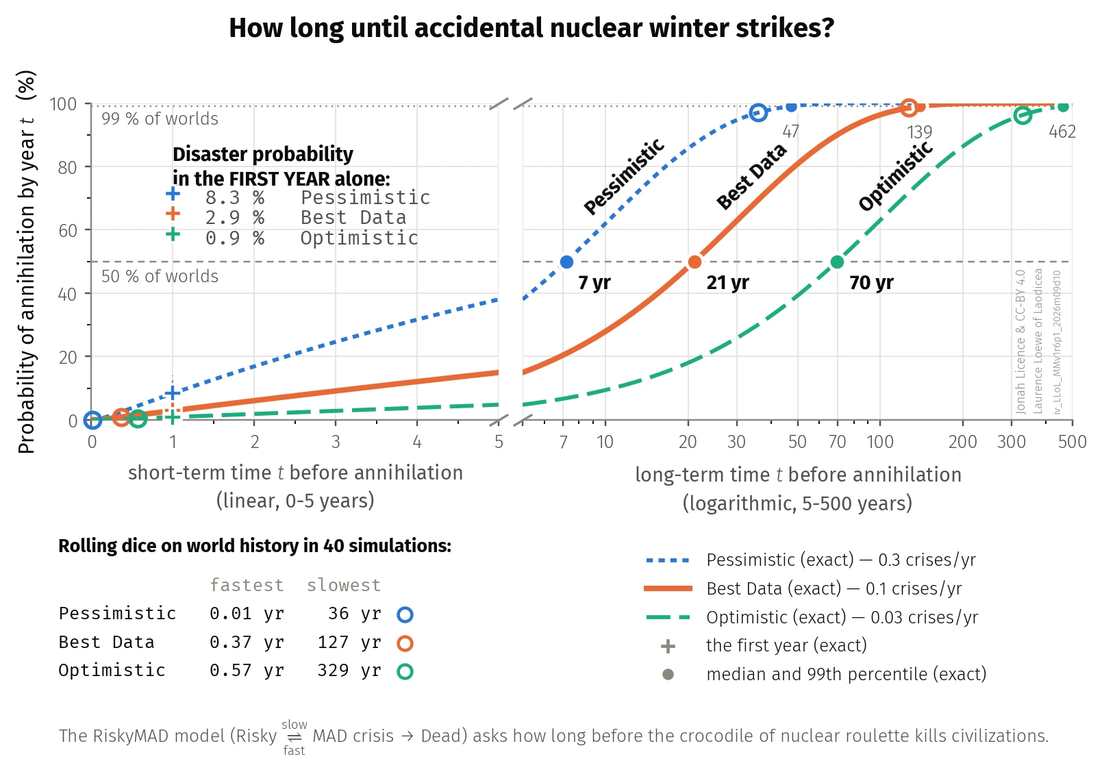
Figure 1: the exact waiting-time law, all three scenarios on one axis. Every
curve is \(P(T_{R \rightarrow D} \leq t)\) from the boxed formula above — no
simulation is involved. Left block (0–5 years, linear): the near-term risk,
which is what people quote. The three scenarios differ by a factor of ten in crisis
rate and by not quite a factor of ten in first-year risk — 8.3 %, 2.9 %, 0.9 %
— so in the first years the three worlds are far less different than the argument
between them suggests. Right block (5–500 years, logarithmic): the medians
(7, 21 and 70 years — even the most optimistic published reading of the record
puts the median inside one lifetime) and the 99th percentiles (47, 139 and 462
years, past which only one world in a hundred is still waiting). Crosses mark the
first year; filled circles the exact medians and percentiles; open rings the
fastest and slowest of the forty simulated runs b16 quotes, tabulated beneath
the figure. Each ring is one draw, shown against where the exact law puts it, not a
claim about the distribution — and the fastest of all reached accidental nuclear
winter in 0.01 years, under four days. The axis break is marked on both facing
edges; the two blocks are not one continuous scale, and on the logarithmic block
equal distance is equal ratio, not equal time, which makes the tail look tamer
there than it is. Drawn by
code/riskymad-forecast-of-nuclear-death-probability-x3.py, which imports the
same functions the audit runs on. The script writes three versions of this figure:
the -plain one used here, one with the caption printed into the image for
sending on its own, and a -public one for a general audience that drops the
percentile markers and numerals and the forty-run table. That a lay reader is
better served without them is a stated guess, not a tested finding — said here
rather than left implied, so that anyone who thinks it wrong knows there is nothing
to overturn but an assumption. All three carry the same numbers; every number in
them is written out as plain text in
code/riskymad-forecast-of-nuclear-death-probability-x3-numbers.txt for anyone
who would rather draw their own.#
What the picture is for. It makes one thing visible that the tables do not: the three scenarios disagree enormously about when and hardly at all about whether. Every curve leads to certain self-destruction. That is section What none of this establishes, in a picture — rates set the schedule, not the outcome.
What the two rates are — and what they are not#
The closed form contains two rates that were not put into the model. Understanding what they mean is where most of the insight in this system lives, and it is also where the b16 prose is very slightly loose (b16-extra section 13).
Why the smaller root is the onset rate#
\(r_{\text{onset}} = 0.0331\)/yr is the rate at which the whole system leaks into Dead once the first weeks are past. It is the number that should be compared with published “X percent per year” estimates of nuclear war — not the crisis rate \(r_{R \rightarrow M}\), which is ten times larger and measures something else entirely.
Three nearby numbers are often confused, and the exact relation between them is worth having:
Quantity |
Base-case value |
What it is |
|---|---|---|
\(1/T_{R \rightarrow D} = r_{R \rightarrow M}\,r_{M \rightarrow D}/(r_{R \rightarrow M}+r_{M \rightarrow R}+r_{M \rightarrow D})\) |
0.032967 /yr |
one over the mean wait |
\(r_{\text{onset}}\) |
0.033087 /yr |
the true long-run onset rate |
\(r_{R \rightarrow M}\, p_{M \rightarrow D} = r_{R \rightarrow M}\,r_{M \rightarrow D}/r_{M \rightarrow \text{out}}\) |
0.033333 /yr |
the naive Poisson shortcut |
These three are not equal, and they are always ordered the same way. Since \(r_{\text{onset}} r_{\text{relax}} = r_{R \rightarrow M}\,r_{M \rightarrow D}\) and \(r_{\text{onset}} + r_{\text{relax}} = r_{\text{all}}\), we have \(r_{\text{relax}} < r_{\text{all}}\) and hence \(r_{\text{onset}} = r_{R \rightarrow M}\,r_{M \rightarrow D}/r_{\text{relax}} > r_{R \rightarrow M}\,r_{M \rightarrow D}/r_{\text{all}} = 1/T_{R \rightarrow D}\). And \(r_{\text{relax}} > r_{M \rightarrow \text{out}}\) whenever \(r_{M \rightarrow R} > 0\) — because \(r_{\text{all}} + \sqrt{\Delta} > 2r_{M \rightarrow \text{out}}\) reduces, after squaring, to \(4r_{R \rightarrow M}\,r_{M \rightarrow R} > 0\) — so \(r_{\text{onset}} = r_{R \rightarrow M}\,r_{M \rightarrow D}/r_{\text{relax}} < r_{R \rightarrow M}\,r_{M \rightarrow D}/r_{M \rightarrow \text{out}}\). Therefore, exactly and always:
Two things follow, and both matter for honesty. First, the naive Poisson product \(r_{R \rightarrow M} \cdot p_{M \rightarrow D}\) is a strict upper bound on the true onset rate — so where the shortcut errs, it errs on the alarming side, and correcting it makes the forecast less alarming, not more. Second, the gap is small: 0.74 % between \(r_{\text{onset}}\) and the shortcut, 1.1 % across the whole sandwich. The shortcut is a good rate. What it is not is a distribution — which is the subject of 7.4.
The hazard rises; it does not start at its final value#
The instantaneous risk of onset at time \(t\), given it has not yet happened, is the hazard:
At \(t = 0\) the numerator vanishes, so \(h(0) = 0\). As \(t\) grows the \(e^{-r_{\text{relax}} t}\) terms die away and \(h(t) \rightarrow r_{\text{onset}}\). In between it rises monotonically.
In plain terms: onset cannot happen immediately, because the world must first enter a crisis and the crisis must then run its course. That takes about forty days on average. So the risk in the first weeks is genuinely lower than the long-run rate, and it climbs to that rate within a few months. Numerically: \(h(0) = 0\), \(h(1\,\text{yr}) = 0.033083\), \(h(100\,\text{yr}) = 0.033087\). The approach is essentially complete after one year.
The relaxation rate is not the crisis#
A correction of identification, not of arithmetic
b16 SIA-4 describes \(r_{\text{relax}} = 9.067\)/yr (written \(r_2\) there before 2026m09d08) as “the fast stage, the crisis itself, mean duration 40 days”. That is a helpful picture and it is very nearly right, but strictly the identification does not hold, and a referee who checks it will notice:
the crisis clock is \(r_{M \rightarrow \text{out}} = 9.000\)/yr, mean duration 40.58 days
the fast mode is \(r_{\text{relax}} = 9.067\)/yr, mean 40.28 days
They differ by 0.74 %, and Why the smaller root is the onset rate shows \(r_{\text{relax}} > r_{M \rightarrow \text{out}}\) strictly whenever \(r_{M \rightarrow R} > 0\). Both round to “40 days”, so no published number is affected. But the two exponentials in the closed form are decay modes of the whole system, not the two physical stages of one round.
Here is the cleanest way to see that they are genuinely different decompositions.
The physical decomposition. Let \(n_{MAD}\) be the number of crises before one escalates. Total time waiting in Risky is a sum of \(n_{MAD}\) exponentials at rate \(r_{R \rightarrow M}\); total time spent inside crises is a sum of the same \(n_{MAD}\) exponentials at rate \(r_{M \rightarrow \text{out}}\). Section 8.1 shows each of these totals is itself exponential, with rates \(r_{R \rightarrow M} p_{M \rightarrow D} = 0.03333\) and \(r_{M \rightarrow D} = 3\) respectively — means 30 years and 1/3 year, adding to 30.333. The means are right.
But these two pieces are not independent. They share the same \(n_{MAD}\): a world unlucky enough to need six crises spends longer at both activities. So the variance does not add:
Variance of the waiting time |
value (yr²) |
source |
|---|---|---|
if the physical pieces were independent |
900.11 |
\(1/(r_{R \rightarrow M} p_{M \rightarrow D})^2 + 1/r_{M \rightarrow D}^2\) |
true value |
913.44 |
\(1/r_{\text{onset}}^2 + 1/r_{\text{relax}}^2\) |
implied covariance between the pieces |
+6.67 |
half the difference |
covariance, measured by simulation |
+6.66 |
200,000 runs |
The closed form’s two exponentials are independent — that is what the factorisation of the transform means — but they are a different pair from the two physical stages. Both pairs give the same mean; only the closed-form pair also gives the right spread. This is why the derivation cannot be short-circuited by “just add the waiting and the crisis time as if independent”.
The shifted-exponential picture, and where the shortcut fails#
For \(t\) beyond a few months the \(e^{-r_{\text{relax}} t}\) term is negligible and
With base-case values \(t_0 = 0.1105\) yr = 40.4 days, and expanding the logarithm shows \(t_0 \approx 1/r_{\text{relax}}\) = 40.3 days. So the entire exact law can be described in one sentence:
The whole result in one sentence
The waiting time behaves like an exponential of rate 0.0331 per year that starts about forty days late.
That forty-day delay is why one horizon, and only one, needs the exact law.
horizon |
shortcut \(1-e^{-t/T_{R \rightarrow D}}\) |
exact |
error |
|---|---|---|---|
1 yr |
3.243 % |
2.900 % |
overstates by 11.8 % |
10 yr |
28.084 % |
27.907 % |
+0.18 percentage points |
20 yr |
48.281 % |
48.216 % |
+0.07 pp |
40 yr |
73.251 % |
73.282 % |
≈ 0.03 pp |
At one year the forty days are 11 % of the window, and the shortcut — an exponential fitted to the correct mean — ignores them. Over a decade or more the delay is irrelevant. The one-year figure is the one everyone quotes, and it is the only one the shortcut got wrong.
Across the four scenarios of b16 Table 3 the one-year overstatement is 12.3 %, 11.8 %, 11.5 % and 10.6 % — so “about 11–12 percent”, not “about 12 percent in every scenario” as b16 currently says (b16-extra section 13).
Reported because it is the paper’s own standard
An earlier draft of b16 computed the headline one-year probability with this shortcut and called it exact: 3.24 % (1 in 31) where the true figure is 2.90 % (1 in 34). No conclusion changed. But a paper whose only request is that others check its arithmetic has no standing to make that request until it has checked its own — which is also why this document exists.
Which question is being asked — and what “we are not in a crisis today” is worth#
An objection worth taking seriously: the world has been running for eighty years, so any “start-up” correction is an artefact of where the model happens to start the clock. In reality the system started up long ago.
The objection is half right, and working out which half is instructive — because both halves turn out to be computable, and they give different answers to the question everyone quotes.
Two legitimate starting conditions.
(a) Start from Risky, known. This is what b16 does. It encodes a fact we actually possess: as of today the world is not in an acute nuclear crisis. Onset therefore cannot happen in the next few weeks without a crisis first arriving and then running its course, so the hazard begins at zero and relaxes upward.
(b) Start from the long-run condition. Ask instead for a typical year, with no knowledge of today’s state. The right initial condition is then the quasi-stationary distribution — 98.9 % Risky, 1.1 % already in a crisis.
Under (b) the correction vanishes exactly. Started from the quasi-stationary distribution, the waiting time is precisely exponential at rate \(r_{\text{onset}}\), with no second term at any horizon:
This is the defining property of a quasi-stationary distribution, and it is checked
numerically against the full two-exponential formula in code/crosschecks.py: the two
agree to machine precision at 0.25, 1, 5, 20 and 80 years.
Question |
Law |
\(P(\leq 1\text{ yr})\) |
used by |
|---|---|---|---|
(a) “We are not in a crisis today. What is the chance within a year?” |
two exponentials |
2.90 % |
b16 |
(b) “In a typical year, what is the chance?” |
one exponential, rate \(r_{\text{onset}}\) |
3.25 % |
— |
Three things follow.
1. The relaxation rate is not academic; it is the price of information. The gap between the two rows — 0.35 percentage points, about 11 % of the figure — is exactly what the knowledge “no crisis is running today” buys. Drop \(r_{\text{relax}}\) from the treatment and that knowledge cannot be expressed at all; the model would have to answer question (b) while being asked question (a).
2. b16’s choice is the conservative one, and this was not previously stated. Question (b) is arguably the more natural reading of “the annual probability”, it is simpler, and it gives the larger number. b16 reports the smaller. That is the right instinct for a paper asking to be checked, but it should be said out loud rather than left for a reader to discover — and it answers in advance a critic who suspects the two-exponential machinery of having been introduced to inflate anything. It deflates.
3. It also explains the retired shortcut. The exponential shortcut that an earlier draft used, \(1 - e^{-t/T_{R \rightarrow D}}\), gives 3.24 % — almost exactly row (b). The shortcut was not nonsense; it was the right answer to the wrong question. That is a more useful diagnosis than “it was wrong”, and it is the reason the error was hard to see.
What this does not license
Row (b) is not an alternative headline to be quoted when it suits. The two rows answer different questions, and only one of them is the question a reader asks when they ask “what is the risk now”. Reporting (a) while a crisis is in fact running would understate the risk badly — the hazard from inside a crisis is \(r_{M \rightarrow D} = 3\)/yr, ninety times the long-run rate. The model’s answer depends on the state of the world at the moment it is asked, which is a feature, not an inconsistency.
Onset is certain; only its schedule is uncertain#
The statement#
For any positive escalation rate, however small, the world reaches Dead with probability one.
Proof. Crises keep arriving: since gaps have finite mean, the number of crises by time \(t\) grows without bound as \(t \rightarrow \infty\). Each escalates independently with probability \(p_{M \rightarrow D} > 0\), so the chance that the first \(n\) all fail to escalate is \((1-p_{M \rightarrow D})^{n} \rightarrow 0\). Therefore \(P(\text{onset eventually}) = 1\). ∎
The same conclusion is visible in the closed form: both exponentials in \(P(T_{R \rightarrow D} > t)\) decay, so \(P(T_{R \rightarrow D} \leq t) \rightarrow 1\).
Nothing about this depends on the size of the rates. They set the schedule. They do not set the outcome.
Rates that change over time#
Assumption A3 (constant rates) can be dropped too. If \(r_{R \rightarrow M}(t)\) varies, onset remains certain provided crises keep coming — formally, provided \(\int_0^{\infty} r_{R \rightarrow M}(t)\, dt = \infty\) and the escalation probability does not fall to zero fast enough for \(\sum_i p_i\) to converge. Since b16 SIA-X2 argues that \(r_{R \rightarrow M}\) has been rising, the constant-rate model is conservative in the direction that matters: a rising crisis rate shortens the wait.
The consequence that policy has to face#
Take a risk-reduction programme far more successful than anything achieved in eighty years: ten times fewer crises (\(r_{R \rightarrow M} = 0.01\)/yr) and crises three times less likely to escalate (\(p_{M \rightarrow D} = 1/9\)). Then
A thirty-fold improvement in the schedule — and the destination is unchanged.
The strongest objection to this, answered honestly
“Nine hundred years is not a problem. Take the win.”
That objection deserves a straight answer rather than a dismissal, and the straight answer has two parts.
First, it is right about the size of the prize. Ten times fewer crises would be the greatest achievement in the history of arms control, and this arithmetic says its value is enormous. Nothing here argues against risk reduction; the model quantifies how much good it does.
Second, it is wrong about the kind of thing it is buying. Nine hundred years is a mean under the assumption that the improvement is permanent. No arms-control arrangement in the nuclear age has been permanent. The 1987 INF Treaty lasted 32 years. New START, the last instrument limiting the two largest arsenals, expired on 2026m02d05 with no successor agreed. When an arrangement lapses, the rates return — and the memorylessness of What “a rate” means means the world gets no credit for the quiet years it banked. Risk reduction buys time; only removing the arrow changes the destination.
That is not this paper’s opinion. It is what a first-passage calculation says about an absorbing state, and it is why elimination and risk-reduction are different kinds of measure rather than different amounts of the same one.
SIA-5 — Claude’s statistics table (scenarios and sensitivity)#
All figures come from the exact first-passage distribution (SIA-4), with \(r_{M \rightarrow R} = 6\)/yr, \(r_{M \rightarrow D} = 3\)/yr, per-crisis death probability \(p_{M \rightarrow D} = r_{M \rightarrow D}/r_{M \rightarrow \text{out}} = 1/3\). No figure in these tables is offered as invariant; the claim that is invariant is the inequality of the final column (the car-crash comparison, SIA-9), which holds in every scenario, including the most optimistic.
Scenario |
crisis rate /yr |
mean |
median |
≤ 1 yr |
≤ 10 yr |
≤ 20 yr |
≤ 40 yr |
≤ 80 yr |
x car-crash [1] |
|---|---|---|---|---|---|---|---|---|---|
optimistic (= Tertrais) |
0.03 |
100.3 yr |
69.6 yr |
0.88% |
9.40% |
18.00% |
32.83% |
54.94% |
18x |
base (4-in-40) |
0.10 |
30.3 yr |
21.1 yr |
2.90% |
27.91% |
48.22% |
73.28% |
92.89% |
58x |
(= Lewis et al.) |
0.15 |
20.3 yr |
14.1 yr |
4.30% |
38.68% |
62.60% |
86.09% |
98.08% |
87x |
pessimistic |
0.30 |
10.3 yr |
7.2 yr |
8.34% |
61.99% |
85.71% |
97.98% |
99.96% |
168x |
Sensitivity to the per-crisis death probability. The escalation probability 1/3 is the paper’s softest structural input (SIA-6, SIA-11). Varying it from 1/10 to 1/2 — the full range anyone has proposed, spanning both ends of Kennedy’s estimate — while holding the crisis rate at its base value of 0.1/yr:
per-crisis death prob. |
implied rates |
mean |
median |
P(onset ≤ 1 yr) |
x car-crash |
|---|---|---|---|---|---|
1/10 |
|
100.3 yr |
69.6 yr |
0.96% |
19x |
1/5 |
|
50.3 yr |
34.9 yr |
1.84% |
37x |
1/3 (base case) |
|
30.3 yr |
21.1 yr |
2.90% |
58x |
1/2 (= Kennedy’s upper end) |
|
20.3 yr |
14.1 yr |
4.05% |
82x |
The parameter moves the waiting time, not the direction. Across the whole range the mean wait moves by a factor of five and the car-crash comparison never falls below 19x — so even at 1/10, below anything the paper’s structure or its anecdotal anchor suggests, an individual remains an order of magnitude more likely to die of accidental nuclear winter than in a car crash. And stochastic certainty holds for any death probability above zero (Section 8): the parameter sets the schedule, not the outcome.
SIA-6 — Calibrating the crisis rate, and the 1/3#
Everything in the forecast is either structural or algebra (SIA-4); two numbers must come from the world. This appendix fixes both: the crisis rate \(r_{R \rightarrow M}\), and the per-crisis death probability \(p_{M \rightarrow D} = 1/3\).
These two are not separately identified, and this appendix does not pretend otherwise. Fixing
\(p_{M \rightarrow D}\) at 1/3 is part of what defines which near-disasters count as entries into a
MAD crisis and are therefore counted by rMADcrisisStarts; a higher true per-crisis chance implies a
correspondingly lower effective crisis rate, and the forecast depends on their product. The
trade-off is worked out exactly in b16-extra, section 14.1 — the one place that
does so.
The criterion, fixed before counting. A civilization-threatening nuclear crisis — an entry into the MAD crisis state — is any incident in which at least one nuclear-armed party’s command authority was confronted with a launch/no-launch decision, or in which nuclear weapons were physically brought to the brink of detonation. This criterion was fixed before counting and is applied unchanged below. A criterion adjusted after seeing the count is not a measurement.
The source. Rather than assemble a private list, the paper calibrates against the largest published catalogue: the 60 historical incidents of Baum, de Neufville and Barrett (2018) [Baum et al., 2018]. Using someone else’s data removes one degree of freedom from an exercise that has too many; the classification below is the paper’s own and is the part a reader should attack first.
Incidents are not excursions. This distinction does most of the work. Six of Baum et al.’s sixty entries belong to the same Cuban missile crisis (the crisis itself, the Duluth–Volk bear incident, the B-59 submarine, the Okinawa missile order, the Florida satellite false alarm, and the Penkovsky false warning). The parameter \(r_{R \rightarrow M}\) counts entries into the MAD crisis state, not incidents, so those six contribute one. Lewis et al. (2014) [Lewis et al., 2014] independently list four separate Cuban-crisis entries, corroborating the distinction from outside this paper. A catalogue of sixty incidents therefore does not imply sixty crises, and any calibration that treats it as one overstates \(r_{R \rightarrow M}\) by roughly an order of magnitude.
What the classification returns. Of the sixty, twenty-seven are excluded as peripheral (threat rhetoric, contingency studies, failed non-state acquisition, weapons accidents with no live launch pathway); a further twenty-three are serious but were caught by procedure rather than by human judgment or luck. The remainder, after collapsing the Cuban-crisis entries, are the five excursions of Table 1 — of which four fall inside the forty Cold-War years, giving
# |
Year |
Event |
Explanation — what actually happened |
Why it qualifies |
Cold War? |
|---|---|---|---|---|---|
1 |
1961 |
Berlin Crisis [4] |
The USSR demanded Western forces leave West Berlin. In October, Kennedy considered a first strike: a White House/Pentagon group produced a detailed plan to destroy Soviet second-strike capability by attacking 1,077 targets, after intelligence showed a much larger US arsenal than believed. He gave a speech instead. |
a disarming first-strike plan reached the President’s desk |
yes |
2 |
1962 |
Cuban Missile Crisis |
The reference event. Thirteen days. Internally it contains at least five further incidents (see note below), including the B-59 submarine, whose captain ordered the nuclear torpedo prepared and then, after consulting Vasili Arkhipov and the political officer, surfaced instead (the account, and what is contested in it: SIA-X7). |
launch decisions reached officers with authority; human judgment, not procedure, stopped them |
yes |
3 |
1983 |
Petrov (Serpukhov-15) [2] |
Soviet satellites indicated an incoming US missile launch. Duty officer Stanislav Petrov judged it a false alarm and declined to report it. He was right: sunlight on high cloud. |
a launch indication reached a human whose judgment was the filter |
yes |
4 |
1983 |
Able Archer |
A realistic NATO command exercise simulating nuclear release, during a period when Soviet leadership feared a genuine first strike. Soviet leadership moved to bunkers; nuclear bombers went to runway alert. |
Baum: “how close they were to launching their own attack is unclear” |
yes |
5 |
1995 |
Norwegian Rocket |
A Norwegian scientific rocket matched the flight profile of a submarine-launched missile intended to blind Russian radar by EMP. Russian forces went to full alert and Yeltsin activated the nuclear command suitcase — the only confirmed activation. |
launch authority was physically engaged by a head of state |
no |
– |
1945 |
World War II [3] |
The atomic bombings of Hiroshima and Nagasaki: the only historical instance of nuclear war. |
excluded from the rate — see [3] |
– |
The two published poles, and what each implies. How many incidents count as near nuclear use is contested, and Baum names the dispute: “analysts disagree on how close they were to nuclear war — for example, Lewis et al. (2014) consider them to have come pretty close, while Tertrais (2017) disagrees.” Rather than adjudicate it, this paper reports both poles.
Position |
Count |
Explanation — what they counted |
\(r_{R \rightarrow M}\) (/yr) |
P(onset ≤ 1 yr) |
|---|---|---|---|---|
Tertrais (2017), skeptical |
1 |
37 episodes reviewed; concludes safety mechanisms held throughout, and that only one significant incident has occurred in ~34 years (Black Brant, 1995). Excludes accidents, unauthorized launch, and terrorism by stated scope. |
0.029 |
0.85% (1 in 117) |
This paper, Table 1 |
4 (Cold War) |
Berlin 1961, Cuba 1962, Petrov 1983, Able Archer 1983; criteria fixed before counting; Norwegian Rocket 1995 falls outside the Cold-War window. |
0.100 |
2.90% (1 in 34) |
Lewis et al. (2014), inclusive |
6 (Cold War) |
Their Table 1 lists 13 cases of near nuclear use; collapsed to excursions (four of the thirteen are Cuban-crisis entries) this gives six Cold-War excursions: Cuba 1962, the 1973 Arab–Israeli war, NORAD 1979, NORAD 1980, Serpukhov-15 1983, Able Archer 1983. |
0.150 |
4.30% (1 in 23) |
Lewis et al., whole era |
10 / 77 yr |
Adds the 1991 Soviet coup, Black Brant 1995, Kargil 1999, and the 2001–02 Kashmir standoff. |
0.130 |
3.75% (1 in 27) |
Three things follow. The scenario range of the tables contains both published poles: the optimistic corner (0.03/yr) is Tertrais’s implied rate; the pessimistic corner (0.3/yr) lies above Lewis et al.’s and rests on the non-stationarity argument of SIA-X2, where it is argued rather than cited. The base case is more conservative than Chatham House: Lewis et al.’s reading implies 1 in 23 per year against the base case’s 1 in 34, so a paper adopting the most inclusive published position wholesale would forecast a higher risk than this one. And the disagreement is narrower than it looks: the two poles are separated by a factor of about five in \(r_{R \rightarrow M}\), and — because the car-crash inequality (SIA-9) is robust across that whole span — they are not separated at all on the question the paper actually asks.
The 1/3, and why it is structural rather than measured. When the system enters a crisis, two competing processes race: de-escalation (rate \(r_{M \rightarrow R} = 6\)) and escalation to exchange (rate \(r_{M \rightarrow D} = 3\)), so \(p_{M \rightarrow D} = r_{M \rightarrow D}/r_{M \rightarrow \text{out}} = 1/3\). This is not arbitrary: it is grounded in the three-mode failure pattern (over-Simplify, over-Complicate, over-Reach) formally derived in Matheo-b12 (the OSCR Collapse theorem). A crisis resolves through one of three modes — reduced to a manageable narrative (returns to Risky), buried under diplomatic work-arounds (returns to Risky), or pushed past the point of no return (Dead). Two of three de-escalate, one escalates; hence \(r_{M \rightarrow R} = 6\) (two escape modes at rate 3) and \(r_{M \rightarrow D} = 3\) (one death mode). The equiprobability of the three modes is a modelling assumption, not a derived result — it is the weakest joint in the paper, and SIA-5 shows the direction survives across the full \(p_{M \rightarrow D}\) range from 1/10 to 1/2.
The only empirical anchor is weak, and it brackets rather than corroborates. President Kennedy privately estimated the probability of nuclear war during the Cuban crisis at “somewhere between one in three, and even” (Sorensen, Kennedy, 1965; via Allison and Zelikow, Essence of Decision, 2nd ed., 1999). This is the closest thing to a measurement of \(p_{M \rightarrow D}\) that exists: one participant’s subjective estimate, from inside one crisis, recorded second-hand. Against his range of 1/3 to 1/2, the model’s 1/3 is the low end. Against the historical record read through Laplace’s rule of succession (SIA-11), the model’s 1/3 is roughly 3.7x too high at \(n = 4\). The two available anchors pull in opposite directions; the chosen value sits between them, closer to the one that produces the lower forecast. The parameter is bracketed, not measured, and the paper says so rather than picking the flattering anchor and calling it support.
SIA-7 — Why Michaelis–Menten kinetics matters (the general case)#
In se magna ruunt — great things collapse upon themselves.
—Lucan, Bellum Civile (Pharsalia) I.81 (c. AD 61–65)
That complex magnificence tends to fail suddenly, and under its own weight, is an intuition roughly two thousand years old. It is not this paper’s discovery, and it is not offered here as evidence — a poet’s observation is not a rate. What the ancient version lacks is the two things that would make it usable: a mechanism that says why such failure is sudden rather than gradual, and a number that says how long one should expect to wait. This appendix supplies the first; SIA-8 supplies the second. The reason to record the intuition at all is that it is old and widely shared, which makes the finding below less exotic than it may first appear — and correspondingly harder to dismiss as a modern alarm.
This appendix carries no numbers; SIA-8 carries them. Onset is a two-step scheme: the world must first enter a crisis (Risky → MAD crisis), and the crisis must then commit to exchange rather than resolve (MAD crisis → Dead). A two-step scheme with a reversible first step and a committed second is exactly the Michaelis–Menten form used for enzyme kinetics — substrate binds, then either releases or is converted. Three consequences follow for any positive rates, independent of the calibration:
Saturation. There is a maximum onset hazard — you cannot die faster than the escalation rate \(r_{M \rightarrow D}\) — so the process behaves like a mechanism that can only work so fast.
Long idle stretches. A saturating process that is in its dangerous state a small fraction of the time produces long calm periods as a matter of course, then ends one. Non-observation is the expected behaviour, not evidence of safety.
Memorylessness. No anniversary is a deadline; the wheel is spun afresh each year. That is what makes the risk durable and the intuition about it unreliable.
Why the analogy earns its keep — and it is not an analogy. The value of Michaelis–Menten kinetics has never been that enzymes are simple. An enzyme is a large machine wandering an enormous configuration space, and the details of how it finds and binds its substrate are, in the general case, hopeless to model. The achievement of the treatment is that you do not need them: all that complexity is absorbed into an effective encounter rate, and the waiting time to product follows from that rate and two others. The same structure holds here, and it is the reason this paper can exist. The “configuration space” is the space of historical causal chains — every way the world can arrange itself into a nuclear crisis, which no one can model. It need not be modelled, because the encounter rate can be measured instead, from the record of times the world did in fact enter that state (SIA-6). The near-miss record plays exactly the role a measured \(k_{on}[S]\) plays in enzymology: the empirical stand-in for a mechanism too complex to derive. And the correspondence is not loose — solving the scheme’s own first-passage equations for the rate of reaching Dead returns the Michaelis–Menten rate law at every point, the same function rather than an approximation in a limit (SIA-8 gives the identity and the numbers).
SIA-8 — The Michaelis–Menten numbers (this system)#
The identity, exactly. Solving the first-passage equations (SIA-4) for the rate at which the chain reaches Dead gives
which is identical, at every point, to the Michaelis–Menten rate law
under the reading below. This is not an analogy that holds in a limit; it is the same function.
Michaelis–Menten |
RiskyMAD |
Value |
Meaning here |
|---|---|---|---|
substrate \(S\) |
crisis rate \(r_{R \rightarrow M}\) |
0.1/yr |
how often the world enters a nuclear crisis |
\(K_m\) |
\(r_{M \rightarrow \text{out}}\) |
9/yr |
how fast a crisis resolves, either way |
\(V_{max}\) |
\(r_{M \rightarrow D}\) |
3/yr |
the escalation step — you cannot die faster than this |
\(k_{cat}/K_m\) |
\(V_{max}/K_m = r_{M \rightarrow D}/r_{M \rightarrow \text{out}}\) |
1/3 |
the specificity constant |
commitment to catalysis |
\(p_{M \rightarrow D} = r_{M \rightarrow D}/r_{M \rightarrow \text{out}}\) |
1/3 |
the fraction of crises that go all the way |
The defining property holds exactly: the rate is half-maximal when \(S = K_m\), and here \(v(9) = 1.5 = V_{max}/2\). The system saturates: as \(r_{R \rightarrow M} \rightarrow \infty\), \(v \rightarrow r_{M \rightarrow D}\) — however often crises arrive, the world cannot be destroyed faster than the escalation step permits.
Where this system sits. With \(r_{R \rightarrow M} = 0.1\)/yr and \(K_m = 9\)/yr,
— ninety times below half-saturation. The system is deep in the first-order regime, which is why the simple product \(r_{R \rightarrow M} \cdot p_{M \rightarrow D}\) works at all: it is the low-substrate limit of a saturating law, and it agrees with the exact solution to 1.1 percent. Saturation would require a crisis roughly every six weeks. The model therefore operates where the correspondence is not merely valid but linear — the easy case, and the one most favourable to a sceptical reader.
A consistency check that was not fitted. The parameters \(r_{M \rightarrow R}\) and \(r_{M \rightarrow D}\) were set from the three-mode structure (SIA-6) with no reference to crisis durations. Yet they imply a mean crisis resolution time of \(1/r_{M \rightarrow \text{out}} \approx 40\) days; the Cuban missile crisis lasted thirteen. Those agree to well within an order of magnitude, from a parameter fixed for independent reasons — offered not as confirmation but as the absence of a contradiction that could easily have appeared.
What the quiet years prove. The system spends about one percent of its time in the bound state: \(r_{R \rightarrow M}/(r_{R \rightarrow M}+r_{M \rightarrow R}+r_{M \rightarrow D}) \approx 0.011\). The rest of the time the doomsday substrate is elsewhere and the world looks safe — because it is safe, most of the time. A process quiescent 99 percent of the time and lethal 1/3 of the time it is not will produce long calm stretches as a matter of course: at the base rate the median wait is 21 years, yet roughly one run in forty survives past 127 (both are the same model). An observer inside the long run concludes the risk is small; an observer inside the short one does not; neither observation moves the underlying rate. The non-observation of nuclear war since 1945 is precisely what this model predicts most of the time, and is therefore weak evidence about the parameters — a property of the variance of first-passage times in a saturating two-step scheme, and checkable by running the model.
SIA-9 — The car-crash comparison#
The forecast is made tangible against a mortality risk societies accept without alarm: dying in a motor-vehicle crash. The comparison must be like-for-like — annual probability, per person, death against death — so three quantities are kept distinct.
The baseline. Road traffic kills about 1.19 million people a year worldwide, roughly 15 per 100,000, or \(1.49\times10^{-4}\) per person per year [World Health Organization, 2023]. The paper uses the global figure, because its claim is about most people. The US rate (\(1.22\times10^{-4}\); 40,901 deaths at 12.21 per 100,000 in 2023 [National Highway Traffic Safety Administration, 2024]) is lower than the global average, so using it would inflate every multiplier below — the direction a motivated author would choose, and the reason not to.
The model’s output is not a mortality. RiskyMAD forecasts the annual probability that accidental nuclear winter begins, not the probability that a given individual dies. The two differ by the death fraction
so individual annual mortality is \(P(\text{onset}) \times q_{\text{dead}}\) — and it is this product, not \(P(\text{onset})\), that may be set beside the road-death figure.
Where \(q_{\text{dead}}\) comes from. It is not this model’s output. Xia et al. (2022) estimate that even a small regional exchange (~100 warheads, 5 Tg soot) causes about 2 billion famine deaths within two years, while a full US–Russia exchange (150 Tg) causes over 5 billion [Xia et al., 2022]. Against a world near 8 billion those are \(q_{\text{dead}} \approx 0.25\) and \(q_{\text{dead}} \approx 0.63\). This paper uses \(q_{\text{dead}} = 0.3\), near the low end and corresponding to the smallest exchange anyone models.
Scenario |
P(onset ≤ 1 yr) |
Individual mortality |
Relative to road deaths |
|---|---|---|---|
optimistic (= Tertrais’s implied rate) |
0.88% |
\(2.6 \times 10^{-3}\) |
18x |
base |
2.90% |
\(8.7 \times 10^{-3}\) |
58x |
Lewis et al.’s implied rate |
4.30% |
\(1.3 \times 10^{-2}\) |
87x |
pessimistic |
8.34% |
\(2.5 \times 10^{-2}\) |
168x |
The stress test. Three inputs are chosen rather than measured: the crisis rate, the death fraction, and the baseline. A reader is entitled to suspect that three choices all landing in the paper’s favour is no coincidence — so each is pushed to its least favourable defensible value at the same time.
Input |
Least favourable defensible value |
Why that value is admissible |
|---|---|---|
crisis rate |
0.03/yr (P = 0.88%) |
Tertrais’s own reading of the record — the most sceptical published position (SIA-11) |
death fraction \(q_{\text{dead}}\) |
0.25 |
Xia et al.’s smallest modelled exchange, 100 warheads [Xia et al., 2022] |
baseline |
7.3e-4/yr |
Libya, ~73.4 per 100,000 (2013) — the highest national rate on record, nearly five times the global average [World Health Organization, 2015] [Guinness World Records, 2013] |
What survives the stress test
Against the global baseline, with the most sceptical crisis rate and the lowest published death fraction: 15x. Against the road-death rate of the worst-affected country on record — Libya, at nearly five times the global average — with those same two concessions: 3x.
The inequality holds at every corner, including all three corners at once. It is not rescued by any single input and cannot be attacked by disputing any single input. The multiplier is a range — roughly threefold at the most punishing corner constructible, sixtyfold at base, a few hundredfold at the pessimistic one. The direction does not move.
The scope switch, and why the number of billions does not matter. Individual annual mortality is the only axis on which these two risks are commensurable, which is why the comparison runs there. On every other axis they differ, and every difference runs the same way. A car crash is idiosyncratic: it kills you and perhaps a few others; the world continues, an insurer pays, the institutions that investigate it exist the next morning. Nuclear winter is systemic: it kills you, everyone you know, the institutions, the counterparty, and the investigator. This is why nothing depends on whether the toll is one billion or eight: at \(q_{\text{dead}} = 0.25\) the inequality holds; at \(q_{\text{dead}} = 1\) it holds; only the multiplier moves. A reader who wants to argue about the billions is arguing about a number the conclusion does not use.
The risk is not unpriced. It was priced, and the price was “uninsurable.”
Nuclear war is excluded from essentially every insurance policy written — property, casualty, life — by a standard nuclear exclusion clause [U.S. Government Accountability Office, 2008]. Not because the risk is small, but because it is uninsurable in principle: insurance requires risks that are independent, so a pool can absorb them, and a solvent counterparty who survives to pay. Nuclear winter violates both by construction. The US Treasury told Congress that war insurance “is not a feasible means for handling war losses of the magnitude which might be expected in a nuclear conflict.”
So the profession that prices catastrophic risk for a living has already examined this one and declined it. The inequality in Table 6 is therefore not a claim that actuaries missed something; it is a claim about what happens when a risk is removed from the domain where risk expertise operates — it stops being measured, then stops being mentioned, and then people conclude from the silence that it is small. The government’s own record shows the pattern: asked whether nuclear, biological, chemical and radiological attacks were insurable, the resulting review [U.S. Government Accountability Office, 2008] catalogued the exclusions and the severity but did not estimate the likelihood; frequency was treated as outside the question. That unasked question — how often — is the one this study answers.
Caution
\(q_{\text{dead}}\) is the softest number in this paper, and it is doing real work. Every figure in Table 6 scales linearly with it; it is anchored to Xia et al. [Xia et al., 2022] rather than derived here, and the anchoring is coarse. A reader who prefers a different \(q_{\text{dead}}\) may rescale the final column directly. The inequality against the global baseline survives for any \(q_{\text{dead}} > 0.017\) — computed at the optimistic corner, the one this paper leans on, and roughly fifteen times below the lowest published estimate. (Taken at the base case the threshold would read \(q_{\text{dead}} > 0.004\), which does not hold where the paper actually leans, so the optimistic-corner figure is the honest one.)
SIA-11 — Strongest objections, and known weaknesses#
Where the strongest sceptic and this paper agree is on method. Tertrais (2017) [Tertrais, 2017] closes by proposing that “the conversation between proponents of deterrence and anti-nuclear activists should revolve around the costs and benefits equation,” and asks whether the system is “tolerably safe.” This paper is an attempt to write that equation down and to put a number on “tolerably.” The dispute is not about whether the question is a cost-benefit one — the sharpest critic says it is — but about what the arithmetic returns once it is done.
“In all the incidents, safety mechanisms worked” — the strongest form of the sceptical case. Tertrais’s most forceful argument is not that the world has been quiet (SIA-7 answers that) but that in every documented near-miss one can watch the safeguard engage — dual phenomenology, fail-safe defaults, procedure holding “even in the early 1960s when they were rudimentary.” That is positive evidence of a working system, not mere absence of catastrophe, and it earns a positive answer. The answer is to grant it, and to have already priced only what it leaves behind. The calibration of SIA-6 excludes the twenty-three incidents “caught by procedure” precisely because the system worked in them; they are not counted as entries into the MAD crisis state. What remains — the four Cold-War excursions — are the cases in which procedure did not suffice and the filter was human judgment or luck (Arkhipov, Petrov) or an unresolved question (Able Archer). The forecast is built on the residue after the working system is credited in full. “The system worked” is therefore not a rebuttal of this paper; it is one of its inputs. The disagreement is only over the four times it did not — and whether four in forty years is reassuring.
Tertrais (2017): the strongest published objection. [Tertrais, 2017] argues that mankind has not repeatedly stood “on the brink”, that the absence of any deliberate explosion since 1945 reflects “human prudence and the efficiency of mechanisms devoted to the guardianship of nuclear weapons,” and — most damagingly for a constant-rate model — that “the probability of failure increases markedly with time only if conditions do not change—and conditions do change.” Four responses, in ascending order of force.
His implied rate is already in this paper. One significant incident in thirty-four years is \(r_{R \rightarrow M} \approx 0.029\)/yr; the optimistic scenario uses 0.03/yr, chosen independently and before the comparison was made. The most sceptical published reading and this paper’s most optimistic corner are the same number. The disagreement is not about that corner but about whether it is the right one.
His scope is narrower than this model’s, which is why his rate is a corner and not a centre. His review, he states, “does not cover the risk of an accidental nuclear explosion, an unauthorized launch, or a terrorist act” — but those are additional routes into the same absorbing state, so his count is, if anything, an under-count. Granting it grants the most favourable reading available.
The declining-incident count may be an artifact of declassification. The incidents he counts are the declassified ones; Cold-War material has had thirty extra years to surface. A constant true rate plus a declassification lag produces exactly an apparent decline in known incidents.
Conditions changed in both directions, and he counts only one. Fail-safes improved; so did the ways to fail — cyber intrusion, hypersonic compression, automated decision support (SIA-X2). His argument establishes that some holes were closed, not that the sum is falling.
None of this refutes him. Response (1) grants a great deal: if his reading is right, the answer is the optimistic column — and even that puts individual annual mortality at eighteen times the global road-death baseline (SIA-9). The disagreement between the most sceptical published position and this paper does not reach the paper’s conclusion — which is the strongest thing the paper can say about its own robustness, because it is a statement about a critic’s numbers rather than the author’s.
“A single use need not become Armageddon” — the escalation-staircase objection. Tertrais, following Herman Kahn [Kahn, 1965], argues that the nuclear threshold is not so thin that one use makes the next casual: escalation may be “a staircase where the last stairs are considerably higher,” resistance rising rung by rung, so a limited exchange need not cascade to a global one. If sound, this weakens the model’s collapse of every escalation into the absorbing Dead state, and it is recorded here as a genuine open flank rather than closed by assertion. Three things bound it. First, Dead is nuclear winter, not first use: the absorbing state is crossed at a soot threshold, and Xia et al. (2022) [Xia et al., 2022] find even the smallest modelled exchange (~100 warheads) injects enough soot to cause about two billion famine deaths (SIA-9) — so “limited” and “below the winter threshold” are different claims, and only the second would help a sceptic. Second, the model already carries the distinction: SIA-1 treats limited exchanges that do not trigger a winter as milestones toward normalising one, not as Dead. Third, to rescue the conclusion the staircase must guarantee that escalation halts below the soot threshold every time, indefinitely, across every actor — a stronger and less defensible claim than Kahn’s, and one Tertrais himself declines to make for “North Korea or Pakistan.” The flank is real; the burden it imposes falls on the optimist.
The Laplace re-weighting a reviewer will try. A reader may ask what happens if \(p_{M \rightarrow D}\) is calibrated from the record too, rather than taken from structure (SIA-6). Suppose \(n\) crises met the criterion and none escalated. Under a uniform prior the posterior mean of \(p\) is Laplace’s rule of succession, \(1/(n+2)\); estimating \(r_{R \rightarrow M} = n/T\) over \(T = 77\) years gives an effective hazard
Counting more crises raises \(r_{R \rightarrow M}\) and lowers \(p\), and the effects very nearly cancel: 0.86 percent/yr at \(n=4\), 1.08 at \(n=10\), approaching 1.30 as \(n\) grows without bound — a limit that converges on Hellman’s independently derived ~1 percent (SIA-10). It is reported, not adopted, chiefly because it is a re-weighting, not a measurement: trading a rising \(r_{R \rightarrow M}\) against a falling \(p\) so that they cancel redistributes an assumption rather than adding information. Three further reasons: \(1/T\) is a posterior mean under a flat prior, not a ceiling; the record is weak evidence at \(n=4\) (surviving four crises at \(p=1/3\) has probability \((2/3)^4 = 19.8\) percent); and at \(n=1\) the rule returns \(p = 1/3\) exactly, so if Cuba is treated as singular, Laplace and Kennedy agree to the digit.
“By this logic one must fear everything” — the Pascalian-mugging objection. A reader may turn the decision argument (Section 10) against itself: if any non-zero probability of an unbounded loss compels action, then every speculative catastrophe — a physics experiment, a stray asteroid, an engineered pathogen — makes the same infinite claim, and a civilization heeding them all could do nothing else. The objection is serious, and it is why the paper does not rest on unbounded loss alone. Four features separate this forecast from such a mugging, and a mugging has none of them. (1) The probability is estimated, not asserted — counted from a public claims history (SIA-6), not conjured to make a downside infinite. (2) The mechanism is demonstrated, not speculative — the atomic bombings of 1945 establish that the escalation rate is positive as a matter of record, not hypothesis (SIA-6, WWII note). (3) The loss is bounded and priced, not infinite — the paper sets a finite, dated transition cost (Section 9) against a finite per-year mortality (SIA-9), never against infinity. (4) The exposure is involuntary, collective, and repeated — unlike a wager one may decline, every person is in the cylinder every year regardless of consent. A mugging trades everything against an unfalsifiable, one-off, vanishing chance; this weighs a bounded, checkable premium against a measured, recurring one. The objection rightly rejects the first. It does not touch the second.
Known weaknesses, stated by the authors.
Crisis-rate uncertainty (§7.1). Four excursions in forty years is a small sample; the true rate could be higher (unreported incidents) or lower (selection bias). The scenario range exists because this number is not known to better than a factor of a few. The favourable direction is bounded: if the count is revised up while the survival record is held fixed, the inferred escalation probability falls in step and the product is bounded — an undercount is not a licence for an arbitrarily higher figure. This is a weaker claim than the argument invites, and a stronger position: it cannot be attacked by disputing the count.
The classification is a judgment layer, not data (§7.1b). Two calls should be attacked first: the 1961 Berlin crisis (this paper’s own addition, absent from Lewis et al.) and Petrov (the most famous case and the weakest of the four). Neither carries the forecast: removing Petrov gives three Cold-War excursions, 0.075/yr, and 2.19 percent per year — 1 in 46.
The 1/3 is the weakest joint (§7.3). The forecast reduces to a product of two numbers; the first is counted (SIA-6), the second is not counted at all, and equiprobability of the three failure modes is not implied by their trichotomy. No revision closes this. What the paper does instead is stop the parameter from carrying the conclusion alone: the stress test (SIA-9) pushes it, the crisis rate, and the baseline against the thesis simultaneously, and the inequality still holds threefold. A reader who rejects 1/3 entirely should go to that table, not to this one.
Model simplicity (§7.2). Three states cannot capture dozens of actors, thousands of weapons, or complex escalation ladders. The simplicity is a strength (transparent, auditable) and a weakness (may miss dynamics that change the conclusion).
The death fraction is anchored coarsely (§7.8). \(q_{\text{dead}} = 0.3\) is tied to Xia et al. rather than derived; every mortality figure scales linearly with it, so the ratios in SIA-9 are order-of-magnitude while the inequality against the global baseline survives for any \(q_{\text{dead}} > 0.017\).
Stationarity is assumed in critics’ favour (§7.9). A constant \(r_{R \rightarrow M}\) cannot accommodate both Tertrais (rate falling) and SIA-X2 (rate rising); the scenario range brackets both readings rather than adjudicating between them.
What the model cannot predict (§7.5). Not when a specific crisis occurs, who is involved, or the trigger — only a probability distribution, which is falsifiable. The practical MAP transition mechanism (§7.4), non-Western strategic lenses (§7.7), and the COOP reading (§7.6) are open questions carried downstream to Matheo-b17 and Matheo-b18.
The claim#
The mean waiting time is distribution-free
\(\mathbb{E}[T_{R \rightarrow D}]\) depends on only three numbers:
the mean time between crisis onsets, \(1/r_{R \rightarrow M}\);
the mean duration of a crisis, \(\tau\);
the probability that a crisis escalates, \(p_{M \rightarrow D}\).
It does not depend on the shape of either waiting-time distribution. No exponential assumption, no memorylessness, no Markov property is required.
What this buys, tested against a hostile substitution#
Replace the model’s exponential crisis duration with the actual duration of the Cuban missile crisis — thirteen days, fixed, not random, as unlike an exponential as a distribution can be — and keep only the mean ten-year gap between crises:
against 30.33 years from the full model: a change of 0.7 %. Substituting a fixed gap of exactly ten years between crises changes the mean by nothing at all, since only its mean enters.
Result |
Needs the exponential form? |
If A2 fails |
|---|---|---|
the mean wait (30.3 yr) |
no — means only |
unchanged |
the certainty of eventual onset |
unchanged |
|
the Michaelis–Menten identity |
yes |
becomes approximate |
the median and the full distribution |
yes |
shape moves; ordering of scenarios does not |
\(P(T_{R \rightarrow D} \leq 1\,\text{yr})\) = 2.90 % |
yes, most of all |
this is the figure genuinely at risk |
So the honest summary is a split verdict, and it is more useful than either a defence or a concession. The mean and the certainty are robust to the assumption most readers will attack. The one-year probability — the number most often quoted — is the one that genuinely depends on it. A critic who says “your memorylessness assumption is unrealistic” has landed a hit on 2.90 %, and none at all on 30.3 years or on the certainty result.
What none of this establishes#
This document has checked the arithmetic thoroughly enough that further checking of the arithmetic has close to zero value. It is important to be equally clear about what remains untouched — because a reader who mistakes a well-checked derivation for a well-checked forecast has been misled, and this paper would then have done harm.
The calibration is where the real exposure sits. Every number depends on \(r_{R \rightarrow M} = 0.10\)/yr and \(p_{M \rightarrow D} = 1/3\). These come from b16 SIA-6: \(r_{R \rightarrow M}\) from counting civilization-threatening crises in the historical record against a criterion fixed before counting, and \(p_{M \rightarrow D}\) from a three-outcome structural argument, anchored anecdotally on Kennedy’s own estimate for Cuba. No amount of algebra can support either number. A critical reader should push there, and b16 SIA-6 already names the equiprobability of the three OSCR modes — the structural assumption behind \(p_{M \rightarrow D} = 1/3\) — as “the weakest joint in the paper”.
The model’s shape is a choice. Three states is a decision about what to ignore — limited exchanges, escalation ladders, multi-party crises, the difference between inadvertent and deliberate use. Section 10 shows the mean is robust to a great deal; it says nothing about whether the right three states were chosen.
The death fraction is imported. \(q_{\text{dead}} = 0.3\) comes from the nuclear-winter literature, not from this model, and every “times car-crash” figure is directly proportional to it. Section 14.2 works through what it counts, what it leaves out, and why 0.3 is a floor rather than a central estimate.
And a forecast is not a solution. That this document exists at all should not be read as progress toward preventing the outcome it describes. It is progress toward being able to defend a number — which is a much smaller thing.
Where marginal effort is worth most
Stated plainly, because it is the practical conclusion of the whole audit: further work on the mathematics has low value; work on the calibration has high value. The algebra is now checked four ways and is not going to be overturned. The crisis rate and the escalation probability have been challenged by exactly the published authors b16 cites, and that is where a critical reviewer will go.
The two subsections below are the beginning of that work, not the end of it.
The crisis rate and the escalation probability are not separately identified#
This is the one place the trade-off is worked out
Everywhere else in this paper and in b16 that names the crisis rate or the per-crisis chance points here. The two are a single calibration, and any argument that varies one while holding the other fixed — in either direction — has to answer this section first.
Two of the model’s three inputs cannot be pinned down independently by anything this paper measures, and it is better to say so exactly than to leave a reader to discover it.
The exact statement. From Reading the formula the mean waiting time is
Holding the escalation rate \(r_{M \rightarrow D}\) fixed, the mean depends on the crisis rate and the per-crisis chance only through their product — exactly, not approximately. Any pair with the same product gives the same answer:
crisis rate |
per-crisis chance |
product |
mean wait |
\(P(\leq 1\,\text{yr})\) |
implied crisis duration |
|---|---|---|---|---|---|
0.03 /yr |
1/3 |
0.010 |
100.33 yr |
0.88 % |
40.6 d |
0.05 /yr |
1/5 |
0.010 |
100.33 yr |
0.93 % |
24.3 d |
0.10 /yr |
1/10 |
0.010 |
100.33 yr |
0.96 % |
12.2 d |
0.30 /yr |
1/30 |
0.010 |
100.33 yr |
0.98 % |
4.1 d |
What follows, and it cuts three ways.
First, fixing the chance at 1/3 is what defines the crisis count. The two inputs are a package. Choosing \(p_{M \rightarrow D} = 1/3\) is equivalent to choosing a counting criterion for what qualifies as a “Cuban-Missile-Crisis type” near-disaster: it says the events being counted are those with about a one-in-three chance of running all the way. Set the chance higher, and the same forecast requires a correspondingly higher effective crisis rate; set it lower, and a lower one. Neither number is known on its own; what the calibration has to get right is the product.
Second, this makes the forecast more robust than it looks. A critic who says “1/3 is too high” has not damaged the result unless they also hold the crisis rate fixed — and holding it fixed is itself a choice, because the crisis count was defined by the very criterion being disputed. The claim that has to survive is a claim about one number, not two.
Third, the compensation is exact for the mean and inexact for short horizons. The four rows above agree on the mean to the last printed digit and disagree at one year (0.88 % against 0.98 %, a spread of 11 %), because they imply different crisis durations — 40 days against 4 days — and the short-horizon figures are sensitive to exactly that (The shifted-exponential picture, and where the shortcut fails). So the trade-off is a genuine freedom for the mean and the median, and only an approximate one for the one-year number. The 40-day figure is the one independently checkable against the historical record: real crises last days to weeks, which is what picks out the first row rather than the last.
What the death fraction counts, and what happens after two years#
\(q_{\text{dead}} = 0.3\) deserves more scrutiny than a single imported number usually gets, because every “times car-crash” figure in b16 is directly proportional to it.
The two-year horizon is real, and it is a truncation. The figures in Xia et al. (2022) are deaths by the end of year 2 after the exchange — about 2 billion for the smallest exchange modelled (5 Tg soot, ~100 warheads) and over 5 billion for a full US–Russia exchange (150 Tg). They are not totals. The climate perturbation is not over at two years: the published simulations find effects persisting for a decade or more, with global temperatures still below normal up to fifteen years after the war [Coupe et al., 2019, Robock et al., 2007], and more than twenty-five years of cooling, with unprecedented ozone loss, even for the far smaller regional case [Mills et al., 2014]. Robock found as early as 1984 that snow and sea-ice feedbacks make the cooling longer and larger than in models without them [Robock, 1984] — the mechanism that makes the mortality tail long rather than sharp.
Note
[Mills et al., 2014] models a regional (5 Tg class) conflict, not the full exchange this paper’s Dead state describes. It supports the claim that recovery is slow; it must not be leaned on for large-exchange magnitudes. No peak-cooling figure is quoted in this section, because the argument needs only the duration. All four citations in this paragraph were checked against the papers on 2026-09-24.
So b16’s 0.3 is conservative twice over. It takes the smallest exchange’s figure for a full-exchange scenario, and it stops counting at the two-year mark while the disruption runs an order of magnitude longer. The scenario-matched, same-horizon figure is 0.63. Substituting it would roughly double every multiplier b16 reports — the base-case comparison would move from 58 × the road-death risk to about 122 ×.
Recommendation, not a change
This is stated here, not applied. b16 SIA-9 should say in one clause that 0.3 is a deliberate floor rather than a central estimate, and what the scenario-matched value would do to the table. A paper that quietly uses a conservative input is being careful; a paper that says it is using a conservative input, and shows what the central value would give, is being audited — and only the second is consistent with this study’s own request.
On a permanent ice age. No published simulation known to this draft reports a transition to a self-sustaining glacial state. The modelled excursion is decades long, severe, and reversible; the albedo feedbacks lengthen it without locking it in. This should be checked rather than taken on trust here, and it is the one claim in this section that rests on absence of evidence rather than on a cited result.
And a simplifying assumption worth stating plainly. This study does not distinguish between outcomes at the bottom of the range: total extinction, and a scattered few million survivors restarting from something close to a pre-agricultural baseline, are both Dead. The model’s absorbing state is the irreversible loss of the civilization that built the weapons — b16 SIA-1 already says this, in those words — and nothing in the forecast depends on resolving what happens below that line. It is a real simplification: it means the model cannot speak to recovery, and does not try to. One clause in b16 SIA-1 making the extinction-versus-remnant equivalence explicit would close the last of the ambiguity.
SIA-12 — Reproducibility#
Every input is public and every step is open to inspection. The complete model, the simulation results, and the MAP escape proposal are published on a single-page poster (SD1), designed for maximum transparency.
Where the companion code is. Four Python files sit beside the companion study in the
project repository, at hell/mm/b/16/extra/code/: riskymad_exact.py (the exact
first-passage law — every quantity in the BEST Names index of SIA-1, as a function),
reproduce_tables.py (recomputes every published figure in this paper and reports HELD
or BREACH for each), crosschecks.py (the independent routes, checked against each other
to machine precision), and the figure script that also writes the numbers behind each plot
as plain text. They need nothing beyond the Python standard library, each runs on its own,
and they use the same Explicit names as the Evolvix model above and as the BEST Names
index, so a reader moves between paper, model and code without a lookup table.
Running reproduce_tables.py prints one line per published figure. At the time of
writing it reports 52 of 52 HELD, 0 BREACH — a reader who finds otherwise has found
something worth reporting.
They are deliberately not offered as a web download. A file served from this site carries no version in its address, so updating a script would silently change what a stable link hands back — the “refresh in place” this series refuses everywhere else. The code will instead be deposited as a versioned archive with its own DOI, so that a reader can fetch exactly the version a given result was computed with, and cite it. Until that deposit exists this paragraph is the honest answer: the code is public, in the repository, at the path above.
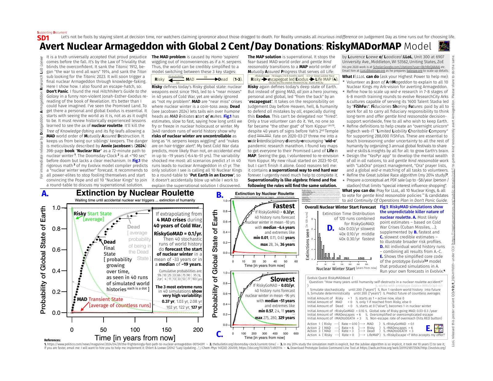
Figure 8: The SD1 poster — full model code, simulation results, and MAP escape path on a single page. Download: SD1.#
To reproduce the simulation results: (1) download the Evolvix prototype compiler from Evolvix Prototype Compiler — Download and RiskyMAD Model Code; (2) enter the model code of SIA-1 (equivalently, from the SD1 poster); (3) run the stochastic simulations; (4) compare against the published forecasts. To check the arithmetic instead, the closed-form first-passage law of SIA-4 needs no compiler at all. The dataset (Baum et al.), the classification criteria (SIA-6, fixed before counting), and every table cell are public, so a reader who rejects a call can strike it and recompute. The code is public, the compiler is public, the results are public. #AuditTheMath.
SIA-13 — Potential-solution details#
The ring (Sections 6 and 9) states the remedy; this appendix supplies the formal apparatus, the concrete specification, and the companion-paper map. Its narrative counterparts — Arkhipov and Gorbachev, the ten Nuclear Kings, Cnut, Earth-in-Escrow — are in Section 6 and are not repeated here.
MAD is metastable, not stable. Mutually Assured Destruction has prevented nuclear war for eighty years, and the model does not deny it; what it adds is one word. A stable equilibrium returns to its state after a perturbation (a ball at the bottom of a bowl); a metastable one looks stable until a large enough perturbation carries it irreversibly past a threshold (a ball on the rim). MAD is the ball on the rim: small crises resolve and the system returns to apparent equilibrium, but the threshold is eventually exceeded — stochastic certainty — and the model measures the basin depth (1 in 34 per year at base, no better than 1 in 113 under the most sceptical reading). This is consistent with the crisis-stability literature (Schelling, 1960; Jervis, 1978), to which the model adds the quantitative result that literature lacks: a distribution over time-to-failure. MAD prevents nuclear war on any given day; it does not prevent it over any given century. A strategy that works locally and fails globally is a delay mechanism.
MAP and the Commitment Trichotomy. Mutually Assured Progress replaces “if you attack, we both die” with “if we both invest in recalibration, we both thrive.” Its formal basis is the Commitment Trichotomy (Matheo-b13, th6): in a Prisoner’s Dilemma cooperation cannot emerge from rational self-interest alone, but a credible first-mover who commits at genuine, irreversible cost converts the game into an Assurance Game, in which cooperation is rational if the other reciprocates.
Side B: Cooperate (reduce) |
Side B: Defect (maintain) |
|
|---|---|---|
Side A: Cooperate (reduce) |
Both reduce risk, save resources. High payoff for both. Mutual progress (MAP). |
Cooperator vulnerable. Worst for cooperator, best for defector. Classic Prisoner’s Dilemma outcome. |
Side A: Defect (maintain) |
Defector gains temporary advantage. Best for defector, worst for cooperator. |
Status quo continues. Stochastic certainty of death for both (Section 8). Both lose over the long term but feel safe locally. Mutual destruction (MAD). |
Three responses exist: defect (the default — assume defection, defect; stable but self-terminating); cooperate naively (exploitable and unsustainable); or volunteer credibly (commit first, at genuine cost, visibly and checkably) — the only one that changes the payoff matrix for everyone else. That third option is not hypothetical: Arkhipov (1962) and Gorbachev (late 1980s) each took it, both Russians, and each “won a world war that never happened” (Section 6). The first-mover payoff already includes the largest reputational prize the international system has — Gorbachev’s 1990 Nobel Peace Prize — paid out once for precisely this move and currently unclaimed. The recalibration mechanism itself is the Jubilee System (Matheo-b14, ax25): every 50 units (7 cycles of 7, plus 1) accumulated imbalances are systematically reset — an engineering specification for a self-correcting civilization, not a utopia.
What MAP looks like concretely. (1) Staged, mutual, verifiable arms reduction — not unilateral disarmament but reduction with checking at every step. (2) Truth-channel restoration as a security measure, since degraded information channels raise the crisis rate. (3) Jubilee cycles applied to international resource allocation — removing the structural conditions that make arms races feel necessary, not redistribution. (4) The Great Jubilee Race: the MAD → MAP transition in 7–8 checkable stages with all ten Nuclear Kings participating. (5) FiShFus (Fiduciaries Sharing Futures): ~288,000 paid long-term thinkers maintaining the “NOT OK” self-assessment the self-correction cycle requires — a civilizational immune system at roughly $8 per person per year (~2 cents per day).
The ten Nuclear Kings — what the term means, and what it does not. “King” is an abstraction for sovereign: the holder of an unappealable decision, answerable to no authority above it. The form of government is irrelevant (presidents, premiers, chairmen, supreme leaders and prime ministers all appear), and “Nuclear” is never dropped. The ten are ten thrones, nine of them armed — the United States, Russia, China, North Korea, India, Pakistan, Israel, France, and the United Kingdom — with Iran included because its declared intention to join means a solution excluding it would not be a solution: intent adds crisis pathways whether or not the warhead exists (SIA-X2), which requires no claim about anyone’s motives. The irony is the point: each is sovereign over his own arsenal and nothing else in this model. The crisis rate is what the world does to him; the per-crisis death probability is what a crisis does once started; and the absorbing state does not check credentials.
Two structural roles for the ten, without which ResearchCity cannot scale. They must permit it, because any one of them could end it: a ResearchCity that will not take up arms is permanently destructible — which is the proposal, not a weakness, because an institution that cannot defend itself cannot become one of the things it was built to correct, and everyone can check that this is so; permitting it therefore costs the ten nothing they would want to keep, which is what makes refusing it informative. They must stay at the table as reviewers, because a solution not transparent to all ten binds none of them: the ten are recruited as reviewers — the same request the paper makes of every reader, addressed to those who hold the classified data that would settle it.
Caveats stated plainly. The symmetric ten-equivalent-Kings model is conservative: real heterogeneity (the US and Russia hold ~90 percent of warheads; China’s no-first-use doctrine; Israel’s opacity; regional India–Pakistan and North Korea dynamics) produces more crisis pathways, not fewer. “Verifiable” is itself a hard problem — arms control has both successes (INF on-site inspection) and failures (Iraq pre-1991, North Korea); the claim is not that checking is easy but that staged checking with milestones is structurally possible and the alternative is worse. And the transition passes through configurations of temporarily elevated uncertainty; that risk is real, but the choice is not “safe status quo versus risky transition” — it is a finite transition risk followed by structural escape, against infinite-horizon certainty of death.
What the escape window costs. The escape transition (rRiskyEscape) is zero not because it is
impossible but because nothing has been built; the escrow window is the interval during which it can be
made non-zero, and Section 9 (Table 8) prices it. A moratorium is not the solution, and calling it one
would be a category error: nothing in a treaty sets the crisis rate to exactly zero (Section 8), and
only that changes the outcome; the window buys building time, not safety. The stages cannot simply be
compressed, because each stage’s checkability depends on the previous one having been checked, so
compression relocates the risk rather than removing it.
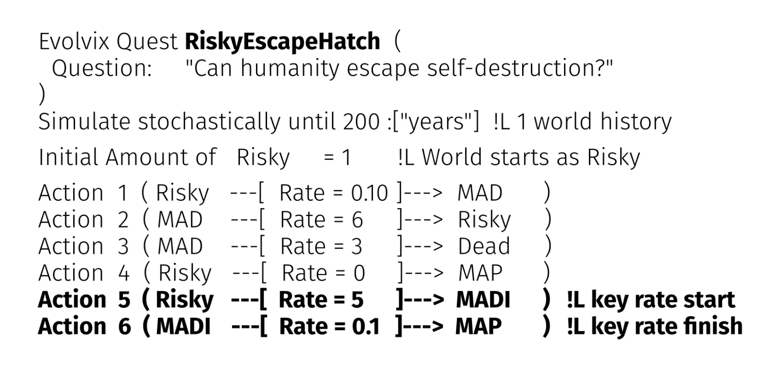
Figure 9: The escape as code, printed beside the base model of SIA-1 so the difference can be
read directly. Actions 1–3 are unchanged: the world still enters a MAD crisis at 0.10/yr, still de-escalates
at 6/yr, still over-reaches to Dead at 3/yr. Action 4 — the direct jump from Risky to MAP —
still carries rate 0: it has never been built. What is added are the two rates the escape actually
turns on, and the code labels them as such: Action 5 opens a route from Risky to MADI (key
rate start) and Action 6 carries MADI on to MAP (key rate finish). The values shown
are illustrative of a built escape, not measured — the point of the figure is that the escape
costs exactly two new lines, and that today both of them are unwritten. #AuditTheMath#
Companion papers. The formal argument is self-contained; the companions supply the axiomatic framework. Upstream: Matheo-b11 (a panentheistic axiom system), Matheo-b12 (the self-correction bifurcation and the OSCR collapse theorem behind the 1/3), Matheo-b13 (the Commitment Trichotomy), Matheo-b14 (the Jubilee System and the Binary Attractor theorem behind SIA-X2), and Matheo-b15. Downstream: Matheo-b17 (falsifiable predictions; who executes the plan and how to test whether they are genuine) and Matheo-b18 (the Call to Action, and the COOP for the MAD → MAP transition). Nothing in the forecast depends on any claim in these: a theological motivation removed a disincentive to measure; it did not supply the measurement (SIA-X5), and the secular reading exists to make that easy to check.
SIA-14 — The scriptural roots of the decision (for those who care)#
Optional depth. Nothing in the main text depends on it — the decision at the centre (Section 5) stands entirely in secular terms. It is set out here, for readers who care, because three of history’s clearest statements of exactly this gate-keeping choice — the life-or-death decision put to a whole people — come from Moses, Joshua, and Jesus, and each maps cleanly onto the secular language used in the ring. It is offered to be tested, not believed.
Moses — the two roads, and why death comes first. “I have set before you life and death … therefore choose life” (Deuteronomy 30:19). This is the decision of Section 5. The single change made in the ring is the order: Moses could say life and death because he was pronouncing a blessing; this paper must say death and life, because in an absorbing-state problem death is the default — the outcome that arrives if nothing is chosen. The inversion is not a correction of Moses; it is the same choice, read from the side of a system that self-destructs unless it is actively steered.
Joshua — the commitment that coerces no one. “Choose you this day whom ye will serve … but as for me and my house, we will serve the LORD” (Joshua 24:15). This is the form of the personal statement in Section 5. Joshua puts the choice to the people and leaves it genuinely theirs, while naming his own answer without hedging — exactly the register the author adopts: a first-person commitment that binds no one else and imposes nothing.
Jesus — why “life by choice” *is* “keep searching, out loud”. Two sayings, read together, supply the content of the secular “life” road. First: “Whoever confesses me before others, I will confess before my Father; whoever denies me, I will deny” (Matthew 10:32–33; Luke 12:8–9). Read as a loyalty test this sounds narrowly devotional; read structurally it is a statement about public commitment — what you are willing to stand behind, in front of others, is what gets carried forward. Second, the name itself. In this series’ dictionary, Yas (the name YhowShua) is read as RealQuestAnswer, from his own words “Who searches will find, and who asks will receive” (Matthew 7:7–8): whoever goes on a real quest will find real answers. The name is the program. So “confessing the name”, stripped to its secular core, is publicly committing to keep searching for the truth — which is what a ResearchCity institutionalises, and what the ring calls “life by choice”.
Jesus — and why the search ends in a Jubilee. His stated mission, at the outset, was to “proclaim the acceptable year of the LORD” (Luke 4:18–19) — in the older law, the Jubilee: the periodic reset that returns what has accumulated in a few hands to everyone (Leviticus 25). That is the second half of the “life” road: a search whose fruits are hoarded curdles back into the thing it replaced, so the same choice carries a Jubilee-based cycle that returns those fruits, on schedule, to all. On this reading the mission was left unfinished — not because the idea failed, but because, by the account, those who could have carried it did not, and abandoned it when it mattered most. The paper’s whole request (Section 6, and Step 0) is that this time enough people do not.
A personal conviction (LLoL) — offered to be tested, not believed
The author states plainly, as personal conviction and not as a result this paper proves: that the life and teaching read here was, for him, what the benzene-ring dream was for Kekulé — the seed of the whole framework — and that he holds the way of Real Quests for Real Answers to be a superior way of understanding the world, and will defend it. This is testimony, not evidence, and it is placed here, in an optional appendix, precisely so that nothing in the paper’s secular argument rests on it. #AuditTheMath applies to it too.
SIA-15 — The decision arithmetic, and why caution lowers the threshold#
Section 9 states the break-even and reports a band. This appendix supplies the derivation, the risk-aversion result the ring only asserts, an independent cross-check by a different method, and the provenance of the numbers. Its limits are separated out into SIA-16, so that a reader who wants the objections can find them whole rather than distributed through the derivation.
What this calculation is called, so nobody has to guess. The frame is a cost-benefit analysis — the benefit is valued in money and set against the cost. The specific move is a break-even (or threshold) calculation: rather than compute a net benefit, solve for the one unknown and ask how small it may be. The rule applied is an expected-value calculation, probability times amount. Only the risk-aversion subsection below is expected-utility theory in the sense axiomatised by von Neumann and Morgenstern [von Neumann and Morgenstern, 1944], and only there is the word utility used. It is not a cost-effectiveness analysis, which compares cost per unit of effect without valuing the effect in money; and it is not what the personnel-selection literature calls “utility analysis”, which is an unrelated procedure that happens to share the word.
The break-even, derived. Let \(K\) be the annual cost per person of the programme, \(r\) the annual probability of onset (Section 4), \(E\) the value one person places on the catastrophe being averted, and \(p\) the probability that the spending in fact averts it. Treating the outcome as all-or-nothing — it is averted or it is not — the expected annual benefit per person is \(p\,r\,E\) and the annual cost is \(K\). Spending is worth making when
Dimensionally \([p] = 1\), \([r] = \mathrm{yr}^{-1}\), \([E] = \$\), so both sides of the first form are dollars per person per year. Worked at the base rate with \(K = 8\), \(r = 0.029\), \(E = 9 \times 10^{5}\): the denominator is \(0.029 \times 9 \times 10^{5} = 26{,}100\) and \(p > 8/26{,}100 = 3.065 \times 10^{-4}\), i.e. 1 in 3,262.8. Substituting \(r/100\) for a hundredfold overstatement gives \(p > 3.065 \times 10^{-2}\), i.e. 3.065 percent. These are the exact values; Table 10 in Section 9 rounds each of them upward — to 1 in 3,000 and 3.5 percent — so that the ring never states a requirement easier than the arithmetic supports (Section 4, on how this paper states its numbers).
A hundredfold overstatement is one operation, and it is well defined
“The danger is overstated a hundredfold” can mean three things, and they agree to within about one percent, so the paper treats them as one move. Dividing the crisis rate \(r_{R \rightarrow M}\) by 100 gives an annual probability of 0.000296 and a median wait of 2,080 years; dividing the annual probability directly gives 0.000290; solving instead for a median of \(100 \times 21.1 = 2{,}110\) years requires \(r_{R \rightarrow M} = 0.000988\) and returns 0.000293. At rates this small the forty-day crisis stage is negligible against the waiting time, so the first-passage law of SIA-4 is effectively linear in \(r_{R \rightarrow M}\) and the knob behaves as one knob.
Why the benefit is credited for one year only. Both sides of the inequality are annual flows, and the comparison is a steady-state one: pay \(K\) this year, and with probability \(p\) avert a hazard that carried probability \(r\) this year. Nothing is credited for the years afterwards, although a hazard actually retired stays retired and the cost of a completed programme would stop being paid. Both simplifications run against the conclusion, which is why they are kept.
For readers who count cautiously: the same question with risk aversion. Everything above prices the loss at its plain money value. Nobody responsible for a catastrophe reasons that way, and neither does the literature on catastrophic risk: a loss that takes everything weighs more than its arithmetic sum, because there is no replacement and no second attempt. The last sack of grain in a famine year is worth more than the thousandth in a good one. This subsection makes that precise, and the result runs opposite to the common intuition that caution makes spending harder to justify.
Setup. Let \(V\) be the reader’s valuation of the state of the world, \(W\) the present state, and let the catastrophe destroy a fraction \(L\) of it — destroyed of the same thing \(E\) is measured against, so that the plain-money stake is \(E = L\,W\). Nothing here requires \(W\) to be wealth; it is whatever the reader was willing to put a number on when setting \(E\). Measure the averted loss in units of value at the margin today, since that is the currency in which \(K\) is paid:
Proposition (parameter-free). For any increasing concave \(V\), \(\widehat{E} \ge E\), with equality exactly when \(V\) is linear on \([W(1-L),\, W]\). Consequently the threshold \(p^{*} = K/(r\widehat{E})\) satisfies \(p^{*} \le K/(rE)\) : risk aversion lowers the required prospect of success. It never raises it.
Proof. Concavity is exactly the statement that a differentiable \(V\) lies below its tangent: \(V(y) \le V(x) + V'(x)(y-x)\) for all \(x, y\) in the domain. Put \(x = W\) and \(y = W(1-L)\), so that \(y - x = -LW\):
Rearranging and dividing by \(V'(W) > 0\) gives \(\widehat{E} \ge L W = E\). Equality holds precisely when the tangent bound is tight across the interval, i.e. when \(V\) is affine there. Since \(p^{*}\) is inversely proportional to the stake, \(\widehat{E} \ge E\) gives \(p^{*} \le K/(rE)\), which is the whole proof.
The consequence worth stating twice. The risk-neutral case is not one point in a range — it is the boundary. Table 10 is therefore a ceiling on the required prospect of success, and every reader who values a catastrophic loss at more than its money sum is entitled to a smaller number than the one printed. That is the durable half of this appendix: it survives any parametrisation, because it never chooses one.
Checked numerically as well as proved. 160,000 random draws of \((W, L)\) across eight concave valuations — square root, logarithm, constant relative risk aversion at \(\eta = 2\) and \(\eta = 5\), linear, \(1 - e^{-ax}\), a quadratic, and a piecewise-linear kink — using exact rather than numerical derivatives, returned a minimum ratio \(\widehat{E}/E\) of 0.999999986. Every value below 1 was traceable to floating-point rounding on the linear cases, where the true value is exactly 1. HELD: no counterexample found.
The standard closed form, for those who want a number. The parameter \(\eta\) below is the relative risk aversion of the valuation, \(-x\,V''(x)/V'(x)\), in the sense of Arrow and Pratt [Pratt, 1964] [Arrow, 1971]. With constant relative risk aversion, \(V(x) = x^{1-\eta}/(1-\eta)\) for \(\eta \ne 1\) and \(\ln x\) at \(\eta = 1\), the ratio evaluates to
At \(\eta = 0\) this returns 1, which is the risk-neutral case and serves as the check. Applied estimates of \(\eta\) cluster between about 1 and 2: Evans (2005) [Evans, 2005] obtains values near unity to somewhat above it across twenty OECD countries, and Groom and Maddison (2019) [Groom and Maddison, 2019] reach a preferred UK figure near 1.5 by four independent revealed-preference routes, with a confidence interval that excludes 1. Nothing in this appendix rests on the choice; the proposition above holds for every value of \(\eta\) greater than zero, and for concave valuations that are not of this family at all.
\(\eta\) |
\(L = 30\%\) |
\(L = 50\%\) |
\(L = 90\%\) |
ceiling at \(L = 50\%\), mid stake ($900,000) |
|---|---|---|---|---|
0 (risk-neutral) |
1.00 |
1.00 |
1.00 |
1 in 3,000 |
1 (logarithmic) |
1.19 |
1.39 |
2.56 |
1 in 4,500 |
1.5 |
1.30 |
1.66 |
4.81 |
1 in 5,400 |
2 |
1.43 |
2.00 |
10.0 |
1 in 6,500 |
Warning
Read the table as illustration, not as measurement. Neither \(\eta\) nor \(L\) is measured here, and a factor table can be made to say almost anything by choosing them. It is printed because a reader is entitled to see the order of magnitude the proposition implies — but the proposition, not the table, is what this appendix asks anyone to rely on. One cell in particular invites misuse: \(\eta = 2\) with \(L = 50\%\) returns a factor of exactly 2, from which it is tempting to say that caution halves the required prospect of success. It does so for that pairing and no other, and nothing measures that pairing. The durable claim here is the direction, not any multiple.
An independent cross-check, by a different method. The break-even above prices a single year at the margin. A second and structurally different route — a multi-year expected-utility comparison of two survival paths — was computed separately and is reported because it agrees where agreement is informative and disagrees where the disagreement is the useful part.
Take one person’s whole position as \(W\), score outcomes by \(\sqrt{\cdot}\) (constant relative risk aversion at \(\eta = 1/2\), the shape economics teaches with), set the horizon at one median wait, count the person’s own life and every descendant at zero, and compare survival while doing nothing against survival if the escape is built halfway through the horizon, at a cost of eight dollars a year. Solving for the prospect of success at which the two are equal:
assumed median wait |
overstatement |
break-even |
as odds |
|---|---|---|---|
20 years (this paper) |
— |
0.039 % |
1 in 2,600 |
50 years |
2.5x |
0.108 % |
1 in 930 |
200 years |
10x |
0.454 % |
1 in 220 |
2,000 years |
100x |
4.6 % |
1 in 22 |
What the comparison shows. At the base case the two methods land within the same order of magnitude — 1 in 2,600 here against 1 in 326 to 1 in 32,628 across the stake band of Table 10, whose middle stake gives 1 in 3,263 — and under a hundredfold discount they give 4.6 percent here against 0.31 to 30.6 percent there. The conclusion is invariant across both. The precise figure is not, and that is why Section 9 reports a band rather than a number: two defensible methods, each internally consistent, differ by enough that quoting three significant figures from either would assert a precision neither has.
Why this appendix reports a band and not a number
The two routes agree where agreement is cheap and disagree where it is informative, and the disagreement is the reason Section 9 quotes bounds rather than figures.
At the observed hazard they land in the same place: 1 in 2,600 by the multi-year route, against a ceiling of 1 in 3,000 at the annual route’s middle stake. Under the hundredfold discount they separate — 4.6 percent against 3.5 percent at that same middle stake, and 0.35 to 35 percent across the full stake band. Both are internally consistent. They differ because they price different things: a single year at the margin against two survival paths over a horizon, with risk aversion built into one and held out of the other as a separate result.
Two defensible methods differing by that much cannot jointly support three significant digits, and quoting either to that precision would assert an accuracy neither has. What both support, and therefore all this paper claims, is the order of magnitude and the direction: a required prospect of success in the thousandths at the observed hazard, and in the low percentages even at a hundredfold discount.
Reproduce either in an afternoon. The annual break-even needs no code. The multi-year route needs this much:
from math import sqrt
W, c, T = 100.0, 100*160/500_000, 20.0      # units of W; c = $8/yr over 20 yr

def threshold(M, eps=0.0, u=sqrt):
    S0, S1 = 0.5**(T/M), 0.5**((T/2)/M)     # survive doing nothing / escape at T/2
    EU0 = S0*u(W) + (1-S0)*u(eps)
    uw, ue = u(W-c), u(max(eps-c, 0.0))
    return (EU0 - (S0*uw + (1-S0)*ue)) / ((S1-S0)*(uw-ue))

for M in (20, 50, 200, 2000):
    q = threshold(M)
    print(f"median {M:>5} yr:  q* = {q*100:7.4f} %   = 1 in {1/q:,.0f}")
What the eight dollars buys, so the figure is legible. At eight billion people, eight dollars a person a year is about 64 billion dollars a year. Two published figures put that in proportion, and one source supplies both: SIPRI records world military expenditure at 2,718 billion dollars in 2024, and puts the global military burden — the share of world output spent on arms — at 2.5 percent [Liang et al., 2025], which fixes world output near 109 trillion dollars without needing a second source. So the programme would cost about one fortieth of world military spending, and about six parts in ten thousand of world economic output. Both roundings run in the direction that over-states the cost (the exact ratios are one in 42.5 and 5.9 in ten thousand), per the rule stated in Section 4. Split across the ResearchCity’s roughly 1,600 units it is about 40 million dollars per unit per year: sixteen hundred ordinary research-institute budgets, which is a quantity a reviewer can weigh against things already funded. The staffing figure behind it — about 288,000 fiduciaries, roughly 180 per unit — is in SIA-13. ((( Both proportions move with the year they are taken from, and 2024 is the latest SIPRI year at the time of writing. )))
SIA-16 — What the decision arithmetic does not establish#
Stated here in one place, at length, so that a reviewer does not have to assemble it and so that nothing below arrives as a discovery. Every item runs against the case Section 9 makes.
It does not establish the hazard rate, and cannot. \(r\) arrives from Section 4 and SIA-6, where it is counted from someone else’s catalogue under a rule fixed before counting. Section 9 assumes that number; it is not a second argument for it. What Section 9 shows is only that if the hazard lies anywhere across a very wide band — two orders of magnitude wide — the decision does not change. That is a reason to pay for the rate to be attacked. It is never a substitute for attacking it.
The stake does not aggregate, and must not be multiplied out. \(E\) is a per-person figure and every term in the inequality is per person; the units check in Section 9 holds only in that form. A reader who multiplies a stake in the millions by eight billion people obtains a total exceeding all world output, which is the well-known arithmetic of aggregating statistical-life valuations and is not a result of this paper. Nothing here requires or implies that total, and no claim below the line is made about what any society could actually afford to spend.
The stake is a value judgement and is left to the reader. What an averted nuclear winter is worth to one person is exactly where values enter, and no arithmetic settles it. Table 10’s band is offered so that a reader can find their own figure inside it and read off the consequence, not as an estimate the paper defends. Any reader who thinks the band wrong replaces one number and recomputes one line — which is the whole reason the calculation was arranged this way rather than as a single result.
It says whether an outlay is worth making, not which outlay is best. Answering the second question would require knowing how the prospect of success grows with spending, and nobody knows that. A decision theorist will see within a minute that the calculation treats \(p\) and \(K\) as independent when they plainly are not. That is a real limitation and it is not repaired anywhere in this paper; what can be said is that the answer does not depend on repairing it, since the threshold is cleared by a wide margin at the one outlay actually costed.
The concavity result is about the valuation of the residual world, not about survival. SIA-15’s proposition holds for any concave valuation of what is left after the catastrophe, with \(L\) the destroyed fraction of whatever the stake was measured against. It is not a result about mortality risk, and it should not be read as one: the literature on valuing changes in survival probability is a separate and harder one, and this paper does not enter it. If a reader sets \(E\) from a statistical-life valuation and then applies a wealth-shaped curvature to it, that reader has mixed two scales, and the factor table of SIA-15 is illustrative at best for them — the parameter-free proposition still holds, because it never asks what the scale is.
The value of being proven wrong is counted at zero. A careful public account of why this forecast fails would retire an urgent claim and redirect the effort it is consuming. That is a real benefit and it is nowhere in the arithmetic. Counting it would make the case for a review stronger, which is precisely why it is left out.
Reviewing is a different question from funding, and an easier one. Section 9 prices the programme. The request in Section 11 is for a review, whose payoff arrives whichever way it comes out — so it is properly a question about the value of information in Howard’s sense [Howard, 1966], what it is worth to find something out before deciding, rather than a break-even on a gamble; and the two should not be conflated. They are easily conflated, because a request to check something and a proposal to fund something can arrive in the same breath and share a price tag. Section 9 prices the programme; Section 11 asks only for the review; and the arithmetic that supports the one is not the arithmetic that supports the other. The distinction is drawn explicitly because a reviewer who notices it before the paper does is entitled to distrust everything nearby.
The Precautionary Principle is deliberately not invoked. It would appear to help and would in fact cost more than it gives. The principle — in German law and usage the Vorsorgeprinzip, and the same thing as the precautionary principle of environmental and European law — licenses action against harms that are conceivable where knowledge is incomplete. This paper is not in that position: it has a rate counted from a claims history and a threshold that can be checked, so it does not need a principle designed for the absence of both, and invoking one would invite exactly the objection SIA-11 answers, that any unbounded downside compels action. The rigorous form of what is actually being used is the distinction between ruin and risk (Section 10) [Taleb et al., 2014]. What this paper borrows instead, and it is not a warrant. A near neighbour of the precautionary principle, easily confused with it and entirely different in purpose, is the Vorsichtsprinzip of German commercial accounting — HGB § 252 (1) no. 4 [Bundesrepublik Deutschland, 1985]. It requires that a balance sheet be valued cautiously: all foreseeable risks and losses must be recognised as soon as they are foreseeable, while gains are recognised only once realised. The asymmetry has a name of its own, the Imparitätsprinzip, and its purpose is that whoever reads the accounts is never surprised in the unfavourable direction.
That is a rule about how to state what you have, not a rule about what to do under uncertainty, which is why it can be borrowed here without borrowing a contested normative claim. Section 4 states the borrowed form: every figure in the ring is a bound that under-claims, every rounding runs against this paper, and the appendices keep the exact values so the discipline can be audited rather than trusted. ((( It is worth being explicit that the two readings of “prudence” point in opposite directions here, and that this paper takes only one of them. Prudence about the danger would mean planning for the worst case. Prudence about one’s own claim means asserting the least the evidence will bear. Only the second is the accounting rule, and only the second is used — which is why the ring quotes the optimistic corner beside the base case rather than the pessimistic one. A paper that used the first while calling it the second would be helping itself to the word. )))
And a limit on what a review is for. The author is not in a position to check his own work: years have gone into it, and confidence built that way is a statement about a person rather than about the world. The two can lie far apart, and this would not be the first time. That is why the request in Section 11 hangs on the weak number rather than the strong one. Nobody is asked to believe that the escape route works. It is enough to hold that it is not ruled out — which is what the threshold above converts into a decision, and it is the least this paper could ask for while asking for anything at all.
SIA-X1 — Why a biologist, and why “top-down”#
Provenance of the forecast, and the modelling philosophy behind it. The ring needs none of this; it is set out for the reader who wants to know who ran the calculation, why, and why its method can be trusted at all. It is numbered X1 so the other appendix numbers stay put; the full set will be renumbered in one pass at the end.
Why a biologist is asking. Loewe is a mechanistic evolutionary systems biologist whose life’s work is Evolvix, a century-stable extensible humane computer-language meant to make accurate modelling in biology simpler — motivated by decades of analysing the complex evolutionary systems biology of real-world organisms. Dreaming that big invites an obvious objection: why spend still more decades defining a language for researchers who may be extinct before it matures? So Loewe’s practical question is also an existential one: will anyone still use computers in a hundred years — enough to justify pushing past “good enough for now”? To decide it, in 2020 he turned the Prototype Evolvix Compiler (REF-LINK) — built while he was an assistant professor, with his lab in a wide interdisciplinary diversity-encouraging (“wid-e”) research centre, in a building “built for a hundred years” (2010) at the University of Wisconsin–Madison, on a US National Science Foundation CAREER grant — onto the forecast reported here. It proved informative enough to settle that original question. It was also so simple that he had to ask why neither he nor anyone he could find had run it before. The rest of this appendix is that answer.
Why not “bottom-up”. Even naming “the right state of mind” among humans is near-certain to start endless argument over what it is and who has it — hence the old advice to avoid religion, politics, sex, and math in polite company. Too many people blindly assume the standing to settle such questions, and the resulting flame wars over symbols have a well-documented habit of becoming literal wars, fought by blindly assuming that leveraging whatever weapon is at hand is a fair way to win the argument. Forecasting such wars from first principles looks hopeless, and for good reason. Centuries of science have shown that the physical world is hard to model accurately; carbon-based biology is immeasurably harder; the information riding human minds is harder still. Bernal (1929) named this rising cascade “the world, the flesh, and the devil”. Even if computers had the right bottom-up structure for every relevant model, estimating the parameters would exceed all the world’s computing capacity: a bottom-up account predicts hyper-astronomically many roads to catastrophe — far too many to enumerate, and far too many to avert one at a time. This paper attempts no better bottom-up model. That would demand intimate knowledge of jealously guarded “national security” secrets the author neither has nor wants; let all the boys keep their secret toys. None of it is needed to see what hides in plain sight — only the patience to build the right top-down model.
Why “top-down” works — the stare at “nothing”. Einstein reportedly credited his breakthroughs less to being cleverer than others than to staying with a problem longer than almost anyone. The “secrets in plain sight” reported here demanded exactly that: a stare at “nothing” long enough that most give up before reaching the narrow, definable path it hides — the mathematically expressible core of how humanity’s self-destruction might be averted. For “nothing” is never quite the same twice; it is whatever should, or should not, be there from a given point of view. Adding what should not be there, or removing what should, can turn a paradise into a hell-scape; adding what should and removing what should not can in principle do the reverse — but only for people who know what they are doing. That instability is the whole difficulty: “nothing is stronger than God” and “nothing is more evil than the devil” use one word for opposite things. A fresh, hard look at “nothing” turns out to matter both for cutting the countless NULL-shaped bugs out of programming languages and for forecasting waiting times to accidental nuclear winter — because it governs how wars are counted. There is a paradise-versus-hell difference between “no disaster” because rivals competed peacefully, as in sport, and “no disaster” because someone like Arkhipov, staring hard at “nothing”, narrowly averted one — winning a world war for all sides at once. Why is there no annual “Arkhipov Day”, on which the world renews its resolve to do the right thing about “nothing” — the most obnoxious advanced persistent threat that can plague any civilization that has not yet learned to defend against it? The claim sounds overwrought; but if the Matheo Study Series (b11–b21, LINKREF) holds up, “nothing” really is such a threat, and this paper — in which “nothing” plays so central and confusing a role — is one exhibit for the point.
Two worked precedents. The confidence that a system this complex can be collapsed to something small comes from having watched it done. The first precedent is from biochemistry: Michaelis–Menten kinetics estimated reaction speeds from simple top-down observation long before anyone could simulate, atom by atom, how an enzyme catalyses a reaction. The same move collapses the complexities of a nuclear-armed world; the details are in the Michaelis–Menten appendix. The second is from complex multiplicative systems such as organisms: Loewe found a long log-normal tail of rare-but-large harmful mutational effects, supported by fruit-fly DNA-diversity data (Loewe 2006), the very shape the law of large numbers produces in multiplicative systems (LOGNORM BOOK-cite). Both are cases where a top-level model earns real, decision-grade traction on a system whose low-level detail is hopeless. Fortunately for this forecast, an evolutionary systems biologist (LINK EvoSysBio 2016) spends a career meeting such cases — watching how “nothing” leaves its traces in real data. Building on that experience, Loewe turned to a system he had grown up with and long dismissed as “boring”.
SIA-X2 — Why the crisis rate increases over time#
The base model assumes a constant crisis rate. This is a conservative simplification; the upstream framework gives formal reasons to expect the rate to increase, which would make the base-case median of ~19 years an upper bound and the model optimistic.
The degradation cascade. The three-mode failure pattern (over-Simplify, over-Complicate, over-Reach; formally derived in Matheo-b12) predicts that any self-assessing system which declares itself “OK” enters a self-reinforcing degradation cycle. Applied to nuclear-armed civilizations: complex geopolitics is reduced to us-vs-them binaries while the truth channels degrade under noise (over-Simplify); arms-control treaties with loopholes and verification regimes with exceptions add work-arounds without restoring the channel (over-Complicate); and a crisis that an earlier era would have managed becomes unmanageable because the correction mechanisms have eroded (over-Reach).
No stable middle. The Binary Attractor theorem (Matheo-b14, th8) holds that there is no stable ground between the self-reinforcing degradation pattern and the active self-correction cycle (Zoning, Investigating, Organizing, Navigating) that counteracts it: scope a problem, examine it honestly, structure a response, steer through implementation, repeat — stopping restarts the degradation. A civilization not actively engaged in that cycle is converging toward the degradation attractor, from which escape becomes harder. Delay is not neutral; it is convergence.
Some holes closed; others opened. Section SIA-11 sets out Tertrais’s argument that the rate is falling — fail-safes perfected, lessons learned, known incidents rare since 1983. That argument is serious and its conclusion is the paper’s optimistic column. But Tertrais’s evidence establishes only that specific failure modes were fixed; it does not establish that the total is falling, because it counts only the closings. Since those fail-safes were designed, the failure surface has changed in kind: command-and-control systems have acquired network attack surfaces that did not exist; hypersonic delivery compresses the decision window that dual phenomenology needs in order to work; and automated decision support inserts a class of error whose failure modes are, by construction, unlike the human ones the existing procedures were built to catch. Whether the sum exceeds the improvements is not known; the claim here is only that it is not obviously negative, and a forecast assuming it is negative is making the stronger assumption.
Pathway growth is quadratic. Bilateral crisis pathways grow as \(\binom{k}{2}\), so nine nuclear-armed states carry thirty-six dyads where five carried ten — a factor of 3.6 in the number of dyads that can produce a crisis, before any account of how much less practised the newer dyads are at managing one. A tenth state is plausible on the current trajectory, though it has not happened and this paper does not forecast it. And each new entrant makes possession more ordinary: a horror that is routine is harder to abolish than one that is shocking, so the crisis rate and the difficulty of reducing it move together, in the wrong direction, for reasons that have nothing to do with anyone’s malice.
The last cap came off in February 2026, and this is not an interpretation. New START — the final treaty limiting the deployed strategic arsenals of the two states holding ~90 percent of the world’s warheads — expired on 5 February 2026, having been extended once (2021) for the five years its text permits, with no further extension legally available and no successor and no negotiations under way [Korda et al., 2026] [International Campaign to Abolish Nuclear Weapons, 2026]. Russia’s verification cooperation had already lapsed in 2023. For the first time since 1972 there is no agreed ceiling on US and Russian strategic forces and no inspection regime attached to one. Treaties constrain arsenals rather than crises, so this does not by itself raise the crisis-rate parameter; what it removes is the transparency and predictability that made crises legible to the other side — the input on which every de-escalation in Table 1 depended. Everything else in this appendix is inference about mechanisms; this is a dated fact with a citation, and it is the kind of evidence the pessimistic column had otherwise lacked.
Caution
What this appendix does not claim. (1) No claim is made about any state’s doctrine, motives, theology, or intentions; the argument is about the number of dyads, the transparency of the channels, and the character of the failure surface — all observable without attributing anything to anyone. (2) Two illustrations that might be expected here are deliberately absent: an assertion about Russia’s stated conditions for use, for which no primary source was located; and a characterization of the 2026 Iran–US–Israel escalation, which the authors cannot check to the standard the rest of the paper is held to. Neither is load-bearing, and current events date quickly: a forecast resting on this year’s headlines deserves the scepticism it will receive.
SIA-X3 — The field report: there is no channel#
SIA-X5 argues that uptake, not analysis, is the binding constraint, and that a forecast delivered without a course of action will be declined. That claim is testable, and the author has been testing it. This appendix reports what came back — as data on the paper’s own uptake hypothesis, falsifiable by a single reply. It is neither a complaint nor a credential nor an appeal: the paper asks for nothing money can buy, and if the uptake hypothesis is right, this outcome is exactly what it predicts.
What was attempted, and what came back. In December 2025, open letters (OL0–OL6, OL10) were sent by post to the Washington representations of the President of the United States, Pope Leo XIV, the Prime Minister of Israel, the President of Russia, the UN Secretary-General, and the US Speaker of the House, and the author travelled to Washington to attempt delivery in person. No response was received from any recipient. The delivery failed at the medium, and that is the finding: the US Secret Service treats unsolicited letters of this kind as spam, and a letter containing a USB stick (how the data travelled) as a security risk; OL10, the most technical of the set, reached no addressee directly at all. The honest finding is not “they were told and ignored it” — it is that there is no channel: the agents whose task is to protect a head of state have no procedure to pass on a claim about an existential risk to the person whose task is to act on existential risks, and the procedures that exist are designed to discard exactly this. Nobody can rebut it by saying they would have read it; the submission was never a thing that could arrive.
Parallel approaches confirmed the shape. Institutions that price risk (banks, including in the course of a legal proceeding) produced no route to anyone with risk-assessment competence — though that test was weaker than it looks, since no actuary was reached, and unnecessary, since the actuarial profession has already answered in writing: nuclear war is excluded by standard clause as uninsurable (SIA-9). Institutions that ought to care (churches, whose own values make catastrophic risk to the whole human family their explicit concern) responded indistinguishably from those with no such commitment. The public responds uniformly “What can I do?” followed by resignation — not apathy but the fourth feature of a super-wicked problem [Lazarus, 2009] [Levin et al., 2012] operating as specified: when a problem seems too large for individual action, discounting the future becomes the rational-feeling default and inaction is chosen without ever being decided (Section 8 explains why inaction is not neutral).
Why there is no channel: a structural reading. The pattern is old and has a name. A system in which the only body empowered to authorize a correction is the body that would be corrected cannot correct itself from the inside — the third defining feature of a super-wicked problem, the central authority needed to address it is weak or non-existent [Lazarus, 2009] [Levin et al., 2012]. At the close of the Middle Ages, Martin Luther observed the same blockage: reform required a council, only the pope could convene one, so errors could be corrected only with the assent of those whose short-term interests the correction opposed. It is cited for the structure and not the man, because it shows the blockage is real, persists for centuries, and is eventually resolved at a cost far exceeding the cost of resolving it early. The nuclear case has the same shape: only the ten can convene the ten — each is party to the matter, none can propose the discussion without appearing to concede something, and there is no authority above them.
But the shape is not identical, and the difference is the opening. Three convening paths exist, not equally exhausted. (1) The United Nations convened the TPNW negotiations in 2017; the nuclear-armed states boycotted and it entered into force in 2021 without them — so its convening power on this precise question has been measured, and the ten do not come. (2) The Holy See signed and ratified the TPNW the day it opened, holds no arsenal, is party to no deterrence relationship, and has stated that possession is immoral [International Campaign to Abolish Nuclear Weapons, 2024] — the only convener that is not also a defendant, and it has not been tried. (3) Any one of the ten could put the waiting-time question on an agenda tomorrow — the strongest path, because under the Commitment Trichotomy (SIA-13) the first credible mover is the mechanism that shifts the game from Prisoner’s Dilemma to Assurance.
The two requests. To whoever convenes: convene. The ask is not that anyone accept this paper’s answer but that the ten be brought to a table to say whether the arithmetic is wrong — if it is wrong, that is the best available outcome, and the fastest route to it is for the people with the classified data to say so; if it is not, they are the only people who can change it. That is why the ten are addressed as reviewers. To everyone else: check the arithmetic, and say what you find. Experts and officials move when there is public interest and, on this evidence, not much before — which makes the smallest available action the operative one. The actionable form of both requests is the ring’s Call to Action (Section 11). #AuditTheMath.
SIA-X4 — Eighty-one anniversaries#
On 6 August 2026 the world marks the eighty-first anniversary of Hiroshima. This paper makes no claim that the date matters. It matters that the date does not matter — which is the whole of SIA-7. The process is memoryless; no anniversary is a deadline; there is no year in which the wheel is not spun. That is precisely what makes the risk durable and the intuition about it unreliable.
What can be said is narrower, and it is not rhetorical. Eighty-one anniversaries have passed, and over that period the crisis rate has not fallen — with reasons to think it has risen (SIA-X2): the nuclear-armed states have grown from five to nine and a tenth is declared; New START expired on 5 February 2026 with no successor and no negotiations under way [Korda et al., 2026], leaving the strategic arsenals of the two largest holders uncapped for the first time since 1972; and the failure surface has acquired cyber intrusion, hypersonic compression of decision windows, and automated decision support, none of which existed when the fail-safes now credited with our survival were designed.
Eighty-one years of quiet is exactly what this model predicts most of the time (SIA-7). It is not evidence that the arithmetic is wrong. It is the reason nobody looks.
SIA-X5 — Why numbers like this go unmeasured#
There is a pattern worth naming, because it bears on how much confidence to place in the absence of forecasts like this one. Risk analysts under-report risks for which they can see no remedy. An unbearable number with no exit attached is one a person finds reasons not to compute — or, having computed it, reasons to temper. This is not an accusation of character but a structural feature of doing risk analysis on a problem one cannot solve, and it predicts exactly what Hellman recorded of himself (SIA-10).
The present author is the stronger case, and it cuts against him. He grew up as the Cold War ended, works on existential problems by profession, and had every modelling tool this paper uses; the model is, by the standards of problems he had already solved, trivially simple — three states, four transitions, a closed-form answer obtainable in an afternoon. He still took years even to look. What changed was not new data or a new method but that a candidate escape (Section 6) had been worked out first, and only then did looking at the number become bearable.
That admission carries an obvious hazard, and it should be stated before a reader states it: if envisioning a solution is what made the problem visible, perhaps the problem was constructed to fit the solution. The reply is evidential, and offered to be checked rather than accepted.
The number does not depend on the escape. Hellman, who has no MAP and no stake in one, reaches ~1 percent per year, within a factor of three of the base case (SIA-10). A preferred solution driving the estimate would not land that close to a man who had no such solution.
The inputs are not this paper’s. The incident catalogue is Baum’s; the classification criteria (SIA-6) were fixed before counting, stated in full, and every cell is recomputable by anyone who disagrees with a call.
The corner most favourable to critics is published here. Tertrais’s reading of the record and this paper’s optimistic scenario are the same number (SIA-11).
A candidate escape removed a disincentive to measure. It did not supply the measurement.
The risk is not unknown. The arithmetic is. That nuclear war would be catastrophic is among the most widely known facts on Earth, public for eighty-one years; the choice to live with it has been made, repeatedly and knowingly, by everyone. What is absent is narrower: a waiting-time distribution — not “this could be very bad” but “here is the probability per year, the median, and what it costs to wait.” Baum finds that nuclear policy decisions “have made little use of risk analysis,” not that anyone is unaware of nuclear war. The two claims must not be run together. The defensible claim is the smaller one: if someone with the background, the motive, the tools, and a three-state model still took years to compute it, it is not reasonable to assume that heads of state — who have none of those four — have been shown a waiting-time forecast. The likeliest explanation for the absence of this calculation from nuclear policy is not that it was weighed and rejected; it is that the number was never put in front of anyone in a form that could be acted on — and SIA-X3 reports what happened when someone tried.
SIA-X6 — Draft status and change record#
This appendix collects the draft-status and provenance notes that would otherwise clutter the top of the paper. It is APPEND-ONLY: new entries go at the bottom, nothing above is rewritten.
Draft status: OOv3r0p0 (2026m07d18) — a soft-ring rewrite of OOv2, not yet reviewed by LLoL. OOv3 carries the same content and the same numbers as OOv2, re-ordered so the decision sits at the centre and all rigour moves into the Supporting Information Appendices (SIAs) at the end. OOv2 is retained, unedited, as a labelled superseded artefact — a record of how AI-assisted work can over-complicate. This working draft holds the full ring (Sections 1–11) and all Supporting Information Appendices (SIA-1–14 and X1–X6); the ring is under active author revision, and the SIAs were ported from OOv2.
What changed between OOv2 and OOv3. Set out in full, with the method used to check that no number moved, in What Changed Between OOv2 and OOv3. In brief: the shape changed (40 nested sections became 11 ring sections plus 19 SIAs), the arithmetic did not, and one block of material was added — a sustained engagement with the strongest published objection, two further objections answered, and six figures. The earlier transition is recorded in What Changed Between MMv5 and OOv2 — that is the revision where the numbers did move.
Front matter (2026m07d25). The title page, author byline, credentials and Declarations footnotes were ported here from OOv2 and stamped to the OOv3 variant, following the Matheo-series title-page convention. The draft-status note that previously sat above the title was moved into this appendix, so the paper opens on its title rather than on its own bookkeeping.
Authorship declarations and References restored (2026m08d03). The OOv2 -> OOv3 port had dropped
the closing Authorship, Contributions, and Declarations section and the .. bibliography::
directive. Without the latter, all 31 :cite: calls in this draft resolved into the reference list
of a different paper (study/matheo/b15/b15-math-deadlock-mmv5) and OOv3 rendered no reference
list of its own. Both are restored below, ported verbatim from OOv2 with only the RST labels
re-stamped oov1- -> oov3- to avoid duplicate-label collisions. The byline, credentials and
identity footnotes 4–7 are NOT repeated here — they already sit on the title page above.
SIA-X7 — B-59, 27 October 1962: the account, and what is contested#
This appendix holds in full, with its sources, the account that Section 1 compresses into one paragraph. It first stood in Section 1 (2026-08-06) and moved here the next day; on 2026-09-24 it was extended by the second, better-recorded crisis of that day and by the crew testimony that records it. The ring needs none of it: the crisis rate is calibrated without B-59 (SIA-6), and the central result survives the sceptic’s reading of the record (SIA-11). It is set out for the reader who wants to know what that paragraph is compressing, who records each step, and — just as important — how much of it is contested and by whom.
A hot steel tube, and the meaning of nothing. In 1962 on Oct 27 — the Saturday on which the Cuban Missile Crisis came closest to ending badly — the Soviet submarine B-59 lay pinned beneath a United States Navy anti-submarine group in the Sargasso Sea, near the American quarantine line. She was a diesel-electric boat built for the North Atlantic, and her cooling had failed on the way out: the diesel coolers blocked with salt, the rubber sealing tore, the electric compressors broke. The carrier USS Randolph headed the group hunting her, and B-59’s own sonar men counted fourteen surface units above them. On the account of her radio-intercept officer, Vadim Orlov, the batteries were flat, only emergency lighting still worked, the compartments stood at 45–50 °C and reached 60 °C in the engine compartment (113–122 °F, and 140 °F), and the carbon dioxide had climbed to what he called “a critical practically deadly for people mark”. Duty officers began going down at their stations — one, then another, then a third, “falling like dominoes”. It went on, he wrote, for about four hours [Orlov, 2002, Savranskaya, 2005].
What was happening above was that the Americans were dropping practice depth charges: hand-grenade-sized signalling devices meant to force a submarine up, not to sink her. The procedure had been published on 24 October to all ships and delivered to the Soviet Foreign Ministry, which promptly handed it back: four or five harmless explosive sound signals meant rise to surface, and a submarine hearing them should surface on an easterly course. That afternoon USS Cony logged: “Challenged submarine contact by dropping five (5) hand grenades” [Burr and Blanton, 2002, Voorhees, 2023]. Whether anybody aboard B-59 knew the procedure is disputed: Savranskaya and Dobbs say the captains did not; Plokhy and Hastings say they did but could not tell practice charges from real ones (the accounts are compared in [Voorhees, 2023]); and the boat’s torpedo officer later called the explosions pre-arranged signals to surface [Leonenko, 2012]. Nor were they the only explosions: the American Julie search system worked by setting off small charges in the water and listening for the echo [Arkhipov, 1997, Mikhailov, 2012], and inside a steel hull one bang sounds much like another. Orlov describes charges that “exploded right next to the hull”, then something “stronger than the grenades … apparently a practical depth bomb”, and a noise like “sitting in a metal barrel, which somebody is constantly blasting with a sledgehammer”. We thought — that’s it — the end. What one side sent as a knock on the door, the other side received as an execution.
The Americans, for their part, did not know what they were prodding. B-59 carried a T-5 torpedo with a nuclear warhead of roughly Hiroshima yield, and so did each of the three other boats in her flotilla. Washington did not know those weapons were at sea at all [Burr and Blanton, 2002].
B-59 did not know what was happening either. A boat of that class could receive Moscow only at or near the surface, and she was having to run too deep to listen. For days, nothing had come in.
That nothing is the hinge of this paper. Silence from Moscow was consistent with two opposite worlds. In one, the crisis was still only a crisis, and the boat’s job was to stay hidden and wait. In the other, the war had already started, their country was already burning, and there was no longer anybody at the far end of the radio. The same nothing fits both. It is not a signal that the world is safe; it is the absence of a signal, and an absence carries no evidence about which of the two worlds produced it.
Nothing else was available either: no orders, no proof, no way to look. Captain Valentin Savitsky — on Orlov’s account, published forty years afterwards — took the worse reading and ordered the nuclear torpedo readied. The words attributed to him are: “Maybe the war has already started up there … We’re going to blast them now! We will die, but we will sink them all — we will not disgrace our Navy.” [Orlov, 2002]
Aboard was Vasili Arkhipov, chief of staff of the 69th Submarine Brigade, riding B-59 by assignment rather than by command. The boat’s commander was Valentin Savitsky, newly appointed to her for this voyage. The two held the same rank, Captain 2nd Rank, and were of an age: Arkhipov, born in 1926, was “essentially a contemporary of the submarine commanders” [Komarov, 2022]. What set him apart was position, not rank, age or command. As the brigade’s chief of staff, second only to the brigade commander (who sailed in B-4), he was the boat’s starshiy na bortu, the “senior officer aboard” for the voyage [Komarov, 2022, Mikhailov, 2012, Savranskaya, 2005]. In Soviet naval usage the phrase names an officer from a higher staff embarked in a ship he does not command. The captain still commanded the boat, and nothing in the sources gives Arkhipov a formal veto. How much his position counted shows in what happened on the surface that night: he gave the order to cancel the dive, and it was obeyed [Leonenko, 2012]. The year before, he had been among the officers who held together the crew of the reactor-stricken submarine K-19. He could not prove that the war had begun. He could not prove that it had not. He was breathing the same foul air, under the same hammering, as ignorant as everybody else in that compartment.
Be careful here, because this is where the famous version and its source part company. The story as usually told has three officers whose agreement was required and one of them refusing. For this afternoon the only witness, Orlov, says something quieter: “we did not fire the nuclear torpedo — Savitsky was able to rein in his wrath. After consulting with Second Captain Vasili Alexandrovich Arkhipov and Deputy political officer Ivan Semenovich Maslennikov, he made the decision to come to the surface” [Orlov, 2002]. No vote, no veto, no single defiant word — a furious, exhausted captain who talked to two colleagues and changed his mind. The vote and the veto were added downstream of that sentence; none of the crew accounts contains them. In an interview Orlov stressed “the crucial role played by the brigade chief of staff Vasili Arkhipov in talking Captain Savitski out of any rash actions” ([Savranskaya, 2005], p. 247), but what Arkhipov said below the surface is not recorded. The quieter version is sourced and, for this study’s purpose, the stronger one. What the argument needs is not a hero but a deliberation — the fact that a decision of this kind turned on whether anybody in that submarine was willing to think straight and say so out loud, and on nothing else.
What broke the tie was not evidence. It was the asymmetry of being wrong. Suppose he was wrong about there being no war, and insisted on surfacing while his country burned: the cost was his boat, his career, and the disgrace of showing a Soviet submarine to the enemy on the surface, unable to dive, in the open. Bad, and survivable — somebody else would still be there to fight the war. Suppose instead the torpedo went and there had been no war: the cost was the war. The two errors were not the same size. One was recoverable and one was not, and that — not any new fact — is the entire argument.
No rule could have supplied that. Notice what was doing the work: not a procedure, but a judgement about which the procedures were silent. No rulebook could have covered this case, and not for want of diligence — covering it would have required writing out, printing, carrying and remembering a library of rules for scenarios that never happened, under conditions in which a rule not remembered is a rule removed. Rules run out exactly where the stakes peak. What has to take over there is the old legal virtue of judging by the purpose of a rule when its letter cannot reach the case — Aristotle’s epieikeia, usually translated as equity or reasonableness. In that compartment it meant two concrete things: extending equal human dignity to the enemy crews the torpedo would have killed, and assigning honest weights to each possible state of an outside world about which no data had arrived for days. That capacity is not a personal virtue this paper hopes for. It is a function, and functions can be staffed, trained and paid for — which is what Sections 6 and 11 eventually ask for.
The third option was to do nothing at all, and this is the part most easily missed. Arkhipov did not have to be right; he only had to speak. The order had already been given. The quiet, safe, blameless course — the one that broke no rule, that nobody would ever have recorded as a decision, and that cost him nothing whatever in the next five minutes — was to say nothing and let the order stand. Doing nothing was not neutral. Doing nothing was the option that ended the world. Cheapest now, fatal later, and invisible as a choice: that combination is the exact shape of the risk this paper prices.
Somebody spoke instead. And then, in an afternoon built entirely out of ambiguous nothings, B-59 did the one unambiguous thing still available to her: “We gave an echo locator signal, which in international navigation rules means that ‘the submarine is coming to the surface.’ Our pursuers slowed down” [Orlov, 2002]. One signal, meaning one thing, under a rule both sides had agreed to in advance — and read correctly, first time, by an enemy in the dark who had spent four hours being misread. The batteries were finished in any case: the commander of her helmsman group and her torpedo officer both say it was the empty battery, not the charges, that brought her up [Leonenko, 2012, Mikhailov, 2012]. She surfaced at 20:52 local time, into the American searchlights [Burr and Blanton, 2002].
The second crisis came on the surface, and it is the better recorded. It is told by two officers inside the boat, the torpedo officer Anatoly Leonenko and the helmsman-group commander Viktor Mikhailov, in memoirs printed in 2012 [Leonenko, 2012, Mikhailov, 2012], and — second-hand, but in print by 2004 — by the captain of the sister boat B-4, Ryurik Ketov [Ketov, 2012]. Savitsky, Arkhipov and a signalman with a portable searchlight went up to the bridge. American aircraft came in low with their searchlights on; the Soviet accounts have them firing ahead of or past the boat, while no American record mentions gunfire and the most thorough sceptic rejects it [Voorhees, 2023]. Savitsky gave the order that instinct gives a submariner under fire: “Urgent dive! Torpedo tubes No. 1 and No. 2, prepare for firing!” Tube 1 held the nuclear torpedo; it had been loaded there before the boat left port [Leonenko, 2012]. In the scramble for the hatch the signalman jammed with his searchlight in the shaft — the accounts differ on who was held up behind whom — and Arkhipov was still on the bridge. He saw an American ship calling them by lamp, and cancelled the dive: “The chief of staff, noticing that the American frigate had begun calling us by searchlight, gave the command to cancel the dive” [Leonenko, 2012]; “The chief of staff, Captain 2nd Rank Arkhipov, gave the command: belay the dive, signalman to the bridge” [Mikhailov, 2012] (both translated from the Russian). The American side of the same minutes survives in a pilot’s report written that December: the destroyers “also used a signal light to ask the contact if he needed any assistance” ([Burr and Blanton, 2002], doc. 47). B-59 answered by lamp that she belonged to the USSR and asked for an end to the provocation, and the aircraft broke off.
Arkhipov’s own account names the mechanism he stopped. Asked in 1997 why the submarine had not used its weapons, he answered that at the first cannon shot the commander “could have instinctively, without contemplation ordered an ‘emergency dive’; then after submerging, the question whether the plane was shooting at the submarine or around it would not have come up in anybody’s head. That is war.” [Arkhipov, 1997]. He did not say that he was the one who stopped it: in his telling the searchlights blinded the commander until “it became clear that the plane was firing past and along the boat”. Mikhailov, writing later, was less modest on his behalf: some minutes had separated them from using a nuclear torpedo against American ships, and only thanks to Arkhipov’s composure had the world avoided a nuclear conflict [Mikhailov, 2012]. A Russian naval historian who quotes the memoirs in full reaches the same verdict — the brigade chief of staff “did indeed show composure and defuse the situation” — and explains why no document will ever confirm the order: the pencil rough log was destroyed on schedule, and no captain would let a breach of the nuclear-use procedure into the fair log ([Komarov, 2022], p. 175).
The standing rule shows why the moment mattered. Before departure the fleet’s chief of staff told the captains to use the special weapon in three cases, one of them if you surface, they fire on you, and you are holed ([Savranskaya, 2005], p. 240; [Ketov, 2012]). A surfaced boat that believed it was under fire was therefore inside the rules for its nuclear torpedo. The dive would not by itself have fired the torpedo — the launch procedure required three keys, and on the best evidence the weapon was never armed ([Savranskaya, 2005], p. 252) — but it would have taken the boat back into the silence where, as Arkhipov put it, nobody could any longer ask whether the fire had been aimed at them.
B-59 charged her batteries under escort, broke contact a few days later, and stayed at sea for about another month before she was ordered home [Leonenko, 2012, Orlov, 2002].
Then nothing happened, and the nothing lasted forty years. There was no headline, because there was no event. The reward for making the right call under about the worst conditions a human being can be given was that the world did not notice, and could not: the evidence of what was prevented is precisely the absence of what was prevented. That Soviet submarines had carried nuclear torpedoes into the quarantine at all became widely known only at a conference in Havana in 2002 — four years after Arkhipov died [Burr and Blanton, 2002]. He never saw the world learn what it had been spared. In the one public statement he made about that day, in Moscow in 1997, he asked why the submarine had not used its weapons and answered without mentioning himself [Arkhipov, 1997]. The one substantial recognition came from a private foundation, posthumously, fifty-five years late, and was collected by his daughter and his grandson [Davey, 2017].
So one word has already done three separate jobs. Nothing was the ambiguous silence he had to read. Nothing was the cheapest thing he could have done about it. And nothing is what a success of this kind looks like from the outside, permanently — which is how a civilization can be repeatedly saved and never find out that it needed saving, and why eighty-one quiet years feel like proof of safety when they are nothing of the kind (Section 7).
Who records what. Nothing numerical depends on this list. It is here so that each step above can be traced to a named witness and checked.
The afternoon order and the decision to surface: Vadim Orlov, the attached radio-intelligence officer, is the only witness, and his accounts shift over time, from no tension at all in 2000 to the full scene in 2002 [Orlov, 2002, Voorhees, 2023].
The night order and Arkhipov’s countermand: Anatoly Leonenko (torpedo officer) and Viktor Mikhailov (helmsman group), from inside the boat [Leonenko, 2012, Mikhailov, 2012]; Ryurik Ketov, captain of B-4, second-hand, in print by 2004 [Ketov, 2012]. The historians who have read the memoirs accept it, the sceptic Voorhees included: “Arkhipov’s steadiness prevailed” ([Voorhees, 2023], p. 139).
The American signals: the destroyers’ deck logs and the pilots’ narratives, written in 1962 [Burr and Blanton, 2002].
Arkhipov himself: one public statement, in 1997, which does not mention his role [Arkhipov, 1997].
His widow: he told her “how they almost fired a nuclear torpedo at an American destroyer” ([Savranskaya, 2005], p. 247).
Soviet documents: none. The Northern Fleet’s draft debriefing report, published in 2022, is silent about B-59 [Savranskaya, 2022], and the Defence Ministry’s 2022 release held nothing on it [Radchenko, 2024].
Note
A caution, placed here rather than in a footnote. Almost every element of this account comes from memory, not from documents, and a specialist reader will know it. The afternoon rests on one oral source, recorded forty years later and published by a journalist [Orlov, 2002], then translated and given scholarly form by Svetlana Savranskaya [Savranskaya, 2005] — who is thus both the translator of that source and its principal interpreter. The night rests on two crew memoirs printed together in 2012, after a second-hand version was already in print, so they are not fully independent; they differ in small details, which argues against copying [Ketov, 2012, Leonenko, 2012, Mikhailov, 2012]. Tertrais (2017) [Tertrais, 2017] holds that the rules of engagement for the torpedo were not met, that it is unclear any vote took place, and that a fellow officer testified Savitsky “never lost it”. Radchenko (2024) [Radchenko, 2024] puts it flatly: “the evidence is not particularly good for it. It’s all oral history” — adding that when the Russian Defence Ministry declassified Cuban Missile Crisis material in 2022 he looked for confirmation and “there was nothing”, though he immediately qualifies that this “in itself doesn’t prove anything”. The most thorough sceptic, Voorhees (2023) [Voorhees, 2023], compares nine published accounts, rejects the aircraft gunfire, finds that the nuclear torpedo was almost certainly never armed, and credits the peaceful outcome to the multi-key rule and mutual restraint rather than to luck — yet he too concludes that “Arkhipov’s steadiness prevailed”. Stern (2012) [Stern, 2012], working from the American tapes, does not name Arkhipov at all: in his telling the captain reconsidered, or “was finally persuaded to wait by another officer”. His corrective is that several independent things had to go right on that one day, so B-59 was one contingency among them and not the single hinge of history.
And the drift is measurable, and it runs both ways, which is the useful part. Set the popular telling beside the accounts it claims to rest on and the additions become visible one at a time: a required vote of three, a veto, a lone refusal, a single word — none of which appear in any crew account. A fiftieth-anniversary newspaper column can be read as one step of that growth, stating plainly that “the launch of the B-59’s nuclear torpedo required the consent of all three senior officers aboard” and that “Arkhipov was alone in refusing permission” [Wilson, 2012] — neither sentence traceable to any witness. But the record also grew in the other direction. The better-recorded episode, the night countermand, reached print only in 2004 and the crew memoirs only in 2012, so the scholarly accounts of 2002–2008 missed it. Nobody lied either way: the legend is more dramatic than its sources, and the sources are fuller than the first scholarship. That is worth pausing on, because a reader is entitled to ask whether this paper does the same with its own numbers. The answer offered is not a promise but a method: every figure in the paper names the appendix that produces it, from public data, so that any drift can be measured rather than trusted.
Nothing numerical in this paper rests on any of it. The crisis rate is calibrated without Arkhipov — B-59 is one incident inside the single Cuban excursion (SIA-6) — and the central result survives on the sceptic’s own reading of the record (SIA-11). On every account, a nuclear torpedo was at sea on the most dangerous day of the crisis, unknown to the ships hunting it, and it was not fired. The story is illustrating a decision here, not carrying a number. And Stern’s correction, taken seriously, runs toward this paper rather than against it: many independent contingencies on a single afternoon is what a high crisis rate looks like from the inside.
Then notice why the record is thin, because that is the thesis in miniature. It is thin because nothing happened. Catastrophes generate archives; averted catastrophes generate silence and a few contested memories. A civilization that measures only what occurred will systematically under-measure how often it nearly did not survive — and will price the risk accordingly.
References#
Arkhipov, V. A. (1997). Address at the Conference on the Cuban Missile Crisis, Moscow, 14 October 1997. National Security Archive Briefing Book No. 808, document 1, published 3 October 2022. https://nsarchive.gwu.edu/document/29078-document-1-vice-admiral-vasili-arkhipov.
Arrow, K. J. (1971). Essays in the Theory of Risk-Bearing. Chicago: Markham Publishing Company.
Barrett, A. M., Baum, S. D., & Hostetler, K. (2013). Analyzing and reducing the risks of inadvertent nuclear war between the United States and Russia. Science & Global Security, 21(2), 106–133. URL: https://scienceandglobalsecurity.org/archive/sgs21barrett.pdf, doi:10.1080/08929882.2013.798984
Barrett, A. M., Baum, S. D., & Hostetler, K. (2013). Appendix and supplement to “Analyzing and Reducing the Risks of Inadvertent Nuclear War between the United States and Russia”. Science & Global Security, 21(2). Online appendix to Barrett, Baum, and Hostetler (2013). URL: https://scienceandglobalsecurity.org/archive/sgs21barrett_app.pdf
Baum, S. D. (2018). Garrick, B. J. (Ed.). Reflections on the risk analysis of nuclear war. Proceedings of the Workshop on Quantifying Global Catastrophic Risks (pp. 19–50). Los Angeles, CA: Garrick Institute for the Risk Sciences, University of California, Los Angeles. https://gcri.org/publications/research/reflections-risk-analysis-nuclear-war.
Baum, S. D., de Neufville, R., & Barrett, A. M. (2018). A Model for the Probability of Nuclear War. Global Catastrophic Risk Institute. Working Paper 18-1, 8 March 2018. https://gcri.org/publications/research/model-probability-nuclear-war/.
Burr, W., & Blanton, T. S. (2002). The Submarines of October: U.S. and Soviet Naval Encounters During the Cuban Missile Crisis. National Security Archive Electronic Briefing Book No. 75, 31 October 2002. https://nsarchive2.gwu.edu/NSAEBB/NSAEBB75/.
Coupe, J., Bardeen, C. G., Robock, A., & Toon, O. B. (2019). Nuclear winter responses to nuclear war between the united states and russia in the whole atmosphere community climate model version 4 and the goddard institute for space studies modele. Journal of Geophysical Research: Atmospheres, 124(15), 8522–8543. URL: https://doi.org/10.1029/2019JD030509, doi:10.1029/2019JD030509
Davey, T. (2017). 55 Years After Preventing Nuclear Attack, Arkhipov Honored With Inaugural Future of Life Award. Future of Life Institute, 27 October 2017. https://futureoflife.org/2017/10/27/55-years-preventing-nuclear-attack-arkhipov-honored-inaugural-future-life-award/.
Diaz-Maurin, F., & Mecklin, J. (2026). AI for peace: in Rome, Nobel laureates call for disarming AI and nuclear weapons. Bulletin of the Atomic Scientists. Bulletin of the Atomic Scientists, 17 July 2026. Available at https://thebulletin.org/2026/07/ai-for-peace-in-rome-nobel-laureates-call-for-disarming-ai-and-nuclear-weapons/. Reports the Global Nobel Laureates Assembly on Artificial Intelligence and Nuclear War, convened at the Vatican (Castel Gandolfo), 14–16 July 2026. URL: https://thebulletin.org/2026/07/ai-for-peace-in-rome-nobel-laureates-call-for-disarming-ai-and-nuclear-weapons/
Evans, D. J. (2005). The elasticity of marginal utility of consumption: estimates for 20 OECD countries. Fiscal Studies, 26(2), 197–224. URL: https://doi.org/10.1111/j.1475-5890.2005.00010.x, doi:10.1111/j.1475-5890.2005.00010.x
Groom, B., & Maddison, D. (2019). New estimates of the elasticity of marginal utility for the UK. Environmental and Resource Economics, 72(4), 1155–1182. URL: https://doi.org/10.1007/s10640-018-0242-z, doi:10.1007/s10640-018-0242-z
Hellman, M. E. (2008). Risk analysis of nuclear deterrence. The Bent of Tau Beta Pi, 99(2), 14–22. URL: https://www.tbp.org/pubs/Features/Sp08Hellman.pdf
Hellman, M. E. (2021). Scouras, J. (Ed.). Probabilistic risk assessment. On Assessing the Risk of Nuclear War (pp. 85–126). Laurel, MD: The Johns Hopkins University Applied Physics Laboratory. Chapter 4. https://www.jhuapl.edu/sites/default/files/2022-12/Ch4_Hellman.pdf.
Howard, R. A. (1966). Information value theory. IEEE Transactions on Systems Science and Cybernetics, 2(1), 22–26. URL: https://doi.org/10.1109/TSSC.1966.300074, doi:10.1109/TSSC.1966.300074
Jacobsen, A. (2024). Nuclear War: A Scenario. New York: Dutton.
Kahn, H. (1965). On Escalation: Metaphors and Scenarios. New York: Frederick A. Praeger. Frederick A. Praeger, New York, 1965 (xvii + 308 pp.). Borrowable scan at https://archive.org/details/onescalationmeta0000kahn; Taylor & Francis reissue at https://www.taylorfrancis.com/books/mono/10.4324/9781315125565/escalation-herman-kahn.
Kemp, L. (2025). Goliath's Curse: The History and Future of Societal Collapse. New York: Knopf.
Ketov, R. A. (2012). Naumov, V. V. (Ed.). Vospominaniya byvshego komandira podvodnoi lodki B-4 o pokhode B-4 v period Karibskogo krizisa [Recollections of the former commander of submarine B-4 on B-4's voyage during the Caribbean Crisis]. Karibskii krizis. Protivostoyanie. Sbornik vospominanii uchastnikov sobytii 1962 goda. Nika-Profi. In Russian. Online serialization, Parts 9–10: https://vnmazurenko.blogspot.com/2013/01/1962-9.html.
Komarov, M. P. (2022). Podvodniki v Karibskom krizise [Submariners in the Caribbean Crisis]. In Russian. PDF posted by the National Security Archive, 3 October 2022; also online, undated, at https://submarinersclub.ru/books/podvodniki_v_karibskom_krizise/.
Korda, M., Johns, E., Knight-Boyle, M., & Kristensen, H. M. (2026 , February). The Aftermath: The Expiration of New START and What It Means For Us All. Federation of American Scientists.
Lazarus, R. J. (2009). Super wicked problems and climate change: restraining the present to liberate the future. Cornell Law Review, 94(5), 1153–1234. URL: https://scholarship.law.cornell.edu/clr/vol94/iss5/8/
Leonenko, A. V. (2012). Naumov, V. V. (Ed.). Vospominaniya byvshego komandira BCh-3 podvodnoi lodki B-59 o pokhode na Kubu: Kamikadze SSSR [Recollections of the former commander of the mine-torpedo department of submarine B-59 on the voyage to Cuba: “Kamikazes of the USSR”]. Karibskii krizis. Protivostoyanie. Sbornik vospominanii uchastnikov sobytii 1962 goda. Nika-Profi. In Russian. Online serialization, Part 28–29: https://vnmazurenko.blogspot.com/2013/01/1962-28-29.html. The night episode is also quoted in full in Komarov (2022), p. 175.
Levin, K., Cashore, B., Bernstein, S., & Auld, G. (2012). Overcoming the tragedy of super wicked problems: constraining our future selves to ameliorate global climate change. Policy Sciences, 45(2), 123–152. URL: https://doi.org/10.1007/s11077-012-9151-0, doi:10.1007/s11077-012-9151-0
Lewis, P., Williams, H., Pelopidas, B., & Aghlani, S. (2014). Too Close for Comfort: Cases of Near Nuclear Use and Options for Policy. Chatham House (The Royal Institute of International Affairs). Chatham House Report, April 2014. https://www.chathamhouse.org/2014/04/too-close-comfort-cases-near-nuclear-use-and-options-policy.
Liang, X., Tian, N., Lopes da Silva, D., Scarazzato, L., Karim, Z. A., & Guiberteau Ricard, J. (2025 , 4). Trends in World Military Expenditure, 2024. Stockholm International Peace Research Institute (SIPRI). SIPRI Fact Sheet, April 2025. Available at https://www.sipri.org/sites/default/files/2025-04/2504_fs_milex_2024.pdf.
Loewe, L., Scheuer, K. S., Keel, S. A., & others. (2017). Evolvix BEST names for semantic reproducibility across code2brain interfaces. Annals of the New York Academy of Sciences, 1387(1), 124–144. URL: https://doi.org/10.1111/nyas.13192, doi:10.1111/nyas.13192
Mikhailov, V. A. (2012). Naumov, V. V. (Ed.). Vospominaniya byvshego komandira rulevoi gruppy shturmanskoi boevoi chasti podvodnoi lodki B-59 o pokhode na Kubu [Recollections of the former commander of the helmsman group of the navigation department of submarine B-59 on the voyage to Cuba]. Karibskii krizis. Protivostoyanie. Sbornik vospominanii uchastnikov sobytii 1962 goda. Nika-Profi. In Russian. Online serialization, Parts 28–29 and 30–31: https://vnmazurenko.blogspot.com/2013/02/1962-30-31.html.
Mills, M. J., Toon, O. B., Lee-Taylor, J., & Robock, A. (2014). Multidecadal global cooling and unprecedented ozone loss following a regional nuclear conflict. Earth's Future, 2(4), 161–176. URL: https://doi.org/10.1002/2013EF000205, doi:10.1002/2013EF000205
Ord, T. (2020). The Precipice: Existential Risk and the Future of Humanity. London: Bloomsbury.
Orlov, V. (2002). Recollections of Vadim Orlov (USSR Submarine B-59): “We Will Sink Them All, But We Will Not Disgrace Our Navy”. National Security Archive document 29066, released with Electronic Briefing Book No. 75, 31 October 2002. https://nsarchive.gwu.edu/document/29066-7-recollections-vadim-orlov-ussr-submarine-b-59-we-will-sink-them-all-we-will-not.
Parkinson, C. N. (1957). Parkinson's Law, and Other Studies in Administration. London: John Murray.
Pratt, J. W. (1964). Risk aversion in the small and in the large. Econometrica, 32(1/2), 122–136. URL: https://doi.org/10.2307/1913738, doi:10.2307/1913738
Radchenko, S. (2024). `Closer now than ever': Historian Sergey Radchenko assesses Tucker Carlson's claim that U.S.-Russian tensions in Ukraine risk nuclear war more than the Cuban Missile Crisis. \emph Meduza, 4 December 2024. https://meduza.io/en/feature/2024/12/04/closer-now-than-ever.
Robock, A. (1984). Snow and ice feedbacks prolong effects of nuclear winter. Nature, 310(5979), 667–670. URL: https://doi.org/10.1038/310667a0, doi:10.1038/310667a0
Robock, A., Oman, L., & Stenchikov, G. L. (2007). Nuclear winter revisited with a modern climate model and current nuclear arsenals: still catastrophic consequences. Journal of Geophysical Research: Atmospheres, 112(D13), D13107. URL: https://doi.org/10.1029/2006JD008235, doi:10.1029/2006JD008235
Savranskaya, S. V. (2005). New sources on the role of Soviet submarines in the Cuban Missile Crisis. Journal of Strategic Studies, 28(2), 233–259. URL: https://doi.org/10.1080/01402390500088312, doi:10.1080/01402390500088312
Savranskaya, S. V. (2022). The Underwater Cuban Missile Crisis at 60. National Security Archive Briefing Book No. 808, 3 October 2022. https://nsarchive.gwu.edu/briefing-book/russia-programs/2022-10-03/soviet-submarines-nuclear-torpedoes-cuban-missile-crisis.
Stern, S. M. (2012). The Cuban Missile Crisis in American Memory: Myths versus Reality. Stanford, California: Stanford University Press. Stanford Nuclear Age Series. Stanford University Press, 2012 (viii + 196 pp.).
Taleb, N. N., Read, R., Douady, R., Norman, J., & Bar-Yam, Y. (2014). The Precautionary Principle (with Application to the Genetic Modification of Organisms). arXiv:1410.5787 [q-fin.GN], latest version 17 October 2014. Available at https://arxiv.org/abs/1410.5787.
Tertrais, B. (2017). “On The Brink”—really? Revisiting nuclear close calls since 1945. The Washington Quarterly, 40(2), 51–66. URL: https://doi.org/10.1080/0163660X.2017.1328922, doi:10.1080/0163660X.2017.1328922
von Neumann, J., & Morgenstern, O. (1944). Theory of Games and Economic Behavior. Princeton, NJ: Princeton University Press.
Voorhees, T. (2023). The Cuban Missile Crisis at sea—avoidance of nuclear war not left to chance. Naval War College Review, 76(2), 107–146. URL: https://digital-commons.usnwc.edu/nwc-review/vol76/iss2/8/
Wilson, E. (2012). Thank you Vasili Arkhipov, the man who stopped nuclear war. \emph The Guardian, 27 October 2012. https://www.theguardian.com/commentisfree/2012/oct/27/vasili-arkhipov-stopped-nuclear-war.
Xia, L., Robock, A., Scherrer, K., Harrison, C. S., Bodirsky, B. L., Weindl, I., … Heneghan, R. (2022). Global food insecurity and famine from reduced crop, marine fishery and livestock production due to climate disruption from nuclear war soot injection. Nature Food, 3(8), 586–596. URL: https://doi.org/10.1038/s43016-022-00573-0, doi:10.1038/s43016-022-00573-0
Bundesrepublik Deutschland (1985). Handelsgesetzbuch § 252 Absatz 1 Nummer 4: Allgemeine Bewertungsgrundsätze. Official consolidated text at https://www.gesetze-im-internet.de/hgb/__252.html. The provision reads, in part: “Es ist vorsichtig zu bewerten, namentlich sind alle vorhersehbaren Risiken und Verluste … zu berücksichtigen …; Gewinne sind nur zu berücksichtigen, wenn sie am Abschlußstichtag realisiert sind.”.
Guinness World Records (2013). Deadliest Place to Travel by Road. Guinness World Records, "Deadliest place to travel by road": Libya, 73.4 road-traffic deaths per 100,000 (2013), citing the WHO Global Status Report on Road Safety 2015. Available at https://www.guinnessworldrecords.com/world-records/deadliest-place-to-travel-by-road.
International Campaign to Abolish Nuclear Weapons (2024). The Holy See and the Treaty on the Prohibition of Nuclear Weapons. Available at https://www.icanw.org/holy_see.
International Campaign to Abolish Nuclear Weapons (2026). The Expiration of New START: What It Means and What's Next. Available at https://www.icanw.org/new_start_expiration.
National Highway Traffic Safety Administration (2024). Traffic Safety Facts: 2023 Motor Vehicle Crashes — Overview. Available at https://www.nhtsa.gov/data/crash-data-systems.
Nobel Laureate Assembly for the Prevention of Nuclear War (2025). Declaration for the Prevention of Nuclear War. Nobel Laureate Assembly for the Prevention of Nuclear War, Chicago, July 2025. Available at https://nobelassembly.org/declaration/; full text at https://nobelassembly.org/declaration-for-the-prevention-of-nuclear-war-final/.
U.S. Department of Transportation (2021 , 3). Departmental Guidance: Treatment of the Value of Preventing Fatalities and Injuries in Preparing Economic Analyses. March 2021 update. Listed on the DOT site as “Valuation of a Statistical Life Guidance” (page last updated 4 April 2021). Available at https://www.transportation.gov/sites/dot.gov/files/2021-03/DOT%20VSL%20Guidance%20-%202021%20Update.pdf.
U.S. Government Accountability Office (2008). Terrorism Insurance: Status of Coverage Availability for Attacks Involving Nuclear, Biological, Chemical, or Radiological Weapons. U.S. Government Accountability Office. GAO-09-39, U.S. Government Accountability Office, 12 December 2008. Available at https://www.gao.gov/products/gao-09-39; full report PDF at https://www.gao.gov/assets/gao-09-39.pdf.
World Health Organization (2015). Global Status Report on Road Safety 2015. World Health Organization. World Health Organization, Geneva, 2015 (ISBN 978-92-4-156506-6; published 16 October 2015). Reports Libya's road-traffic death rate at 73.4 per 100,000 (2013 data), the highest national rate in the report. Available at https://www.who.int/publications/i/item/9789241565066; full PDF at https://iris.who.int/bitstream/handle/10665/189242/9789241565066_eng.pdf.
World Health Organization (2023). Global Status Report on Road Safety 2023. World Health Organization.