Forecasting Actuarial Waiting Times for Accidental Nuclear Winter#
dv_ClaOp48Max_OOv2r0p0_2026m07d16Broader Significance
Nuclear war is usually argued in words. This study argues it in numbers, using the oldest quantitative discipline built for questions of this shape: actuarial science. An actuary cannot say when a particular person will die. Given a population, a set of risk factors, and a claims history, an actuary can still price the risk — and be wrong in ways that show. This study treats the system of nuclear-armed states as the life being priced, the Cold-War record of near-misses as the claims history, and accidental nuclear winter as the death.
At the rate crises have actually arrived, half of all runs of world history reach accidental nuclear winter within twenty-one years, and the chance it begins in any given year is about one in thirty-four. Set beside a risk that societies accept without alarm — dying in a road accident — a person is roughly sixty times more likely to die as a consequence of accidental nuclear winter than in a car crash, counted the same way: annual, per person, death against death. That comparison is this study’s central claim, and it is built to be attacked rather than admired. It survives when the most sceptical published reading of the record, the lowest published death toll, and the road-death rate of the worst-affected country on record are applied all at once.
This risk is not invisible because it is small. It is invisible because it has been removed from the places where risks are measured. Nuclear war is excluded by standard clause from essentially every insurance policy written: the profession that prices catastrophe for a living examined this one and declined it, on the correct grounds that it is uninsurable in principle — there is no surviving counterparty to pay. It was priced at infinity, and then not spoken of. What follows is not alarm. It is arithmetic, from public data, repeatable in an afternoon.
Readers concerned with nuclear policy, existential risk, actuarial practice, or the governance of problems that no single authority is empowered to correct will find the method and the failure modes relevant. Readers who suspect this of being alarmism should begin at Section 5.3: the most sceptical published critic of nuclear close-call analysis supplies this study’s own optimistic scenario, and the conclusion holds there too. Readers who want the escape without the theology will find it in a companion written in entirely secular terms.
The study is offered not to be believed, but to be checked. If it is wrong, the fastest way to find out is for someone to say so.
Declarations
Note
Draft status: OOv2r0p0 (2026m07d16) — not yet reviewed by LLoL. Successor to the
OOv1 draft, following an adversarial panel review. If you have seen 3.24 percent quoted from
this work, see Section 2.0a: it was too high, by about 12 percent, and in this study’s own
favour. What changed between the MMv5 floor and this draft — what was refined, what
was corrected, and the one claim that was removed — is set out in
What Changed Between MMv5 and OOv1,
with links to the full audit trail. Prior versions mmv1/–mmv3/ are retained
unedited as the archive.
Abstract
How long does a civilization survive with nuclear weapons and without periodic recalibration? This study answers that question the way an actuary prices a life: as a probability distribution over time-to-failure, calibrated on a claims history, and falsifiable against it.
The model. RiskyMAD is a three-state continuous-time Markov chain — Risky (weapons exist, no exchange), MAD (a crisis in which nuclear use is on the table), and Dead (accidental nuclear winter, an absorbing state). Four transitions connect them. The chain is small enough to solve exactly, and the exact first-passage law is derived here rather than approximated: it is hypoexponential, the sum of two exponentials, because a crisis takes time to resolve before onset is possible at all.
The calibration. The one parameter that must come from the world is the rate at which civilization-threatening nuclear crises arise. It is counted here from the largest published catalogue of such events — the sixty incidents compiled by Baum, de Neufville and Barrett (2018) — under a criterion fixed before counting. Incidents are not excursions: six of their sixty belong to the single Cuban missile crisis and contribute one entry. The classification returns four Cuba-grade entries in the forty Cold-War years, a crisis rate of 0.1 per year. The probability that a crisis escalates rather than de-escalates is taken as 1/3, from a structural argument, bracketed by Kennedy’s contemporaneous estimate of “between one in three, and even” on one side and Laplace’s rule of succession on the other.
The results. At the base rate, the mean time to onset is 30.3 years and the median is 21.1 — half of all runs of world history are over within twenty-one years. The annual probability that accidental nuclear winter begins is 2.90 percent, about 1 in 34; over forty years, one career, it is 73 percent. Across a scenario range bracketing both published poles of the near-miss literature, the annual probability spans roughly 1 to 8 percent. Forty stochastic simulations of world history agree with the closed form to within sampling noise.
The comparison. Discounted by a death fraction taken from the nuclear-winter literature, individual annual mortality from accidental nuclear winter is roughly fifty-eight times the global road-death baseline, counted annual-per-person against annual-per-person. The inequality holds in every scenario, and it holds by threefold when the most sceptical crisis rate, the lowest published death toll, and the highest national road-death rate on record are imposed simultaneously.
The mechanism, and why eighty-one quiet years prove little. The scheme is a saturating two-step process of exactly the Michaelis–Menten form, and the world sits ninety times below half-saturation: the system is in its lethal state about one percent of the time. A process like that produces long calm stretches as a matter of course. Non-observation of nuclear war since 1945 is what this model predicts most of the time, and is therefore weak evidence about the rate.
What the study does not claim. The classification of Baum et al.’s incidents is this study’s own, and is the part a reader should attack first; two calls are named in advance as weakest, and removing the most contested gives 1 in 46 rather than 1 in 34. The escalation probability of 1/3 is not measured, and no revision closes that gap. The absorbing state is not resolved to a warhead count.
The escape, and its price. Because the Dead state is absorbing, accidental nuclear winter is a stochastic certainty under business as usual: the only open question is when. The study derives a candidate escape — MAP, Mutually Assured Progress — in which a credible first-mover converts the nuclear Prisoner’s Dilemma into an Assurance Game. It then prices that escape with the same model: a seven-to-eleven-year transition carries a 20 to 30 percent chance of not finishing in time, against 73 percent over a career of doing nothing.
Every input is public and every step is open to inspection. The dataset is not this study’s own; the equations are in Section 2.4a; the classification is tabulated incident by incident so that a reader who rejects a call can strike it and recompute. Don’t believe it — #AuditTheMath.
1. The Question#
How long does a civilization survive with nuclear weapons and without periodic recalibration?
This is not a philosophical question. It is a stochastic modeling question — the same kind of question an actuary asks when pricing a life insurance policy. An actuary does not know when a particular person will die. But given a population, a set of risk factors, and historical data, the actuary can estimate a probability distribution over time-to-death. The estimate is falsifiable: if the actual death rate deviates significantly from the predicted distribution, the model is wrong and must be revised.
This paper applies the same logic to nuclear civilization. The “patient” is the global system of nuclear-armed states. The “risk factor” is the rate at which crises arise that bring the system to the brink of nuclear war. The “historical data” is the Cold War record of near-misses. The “death” is accidental nuclear winter — not a deliberate nuclear strike, but the unintended initiation of nuclear exchange through miscalculation, system failure, or escalation beyond the point of human control, and the subsequent global catastrophe as nuclear winter kills far more people than the initial exchange.
The question is not whether accidental nuclear winter is possible. The Cuban Missile Crisis (1962), the Able Archer exercise (1983), Stanislav Petrov’s false alarm (1983), and Vasili Arkhipov’s refusal to authorize a nuclear torpedo (1962) have already answered that question. The question is: given the observed crisis rate, what is the probability distribution over the time until accidental nuclear winter begins?
This is not an idiosyncratic worry. In July 2025 the Nobel Laureate Assembly for the Prevention of Nuclear War warned that nuclear war is uniquely able to end civilization “in an afternoon” [Nobel Laureate Assembly for the Prevention of Nuclear War, 2025]; a year later, convened at the Vatican, the Global Nobel Laureates Assembly on Artificial Intelligence and Nuclear War warned that “AI built into nuclear systems leaves little time for, or even replaces, human judgement in a crisis” [Diaz-Maurin and Mecklin, 2026] — the exact failure this model takes as its absorbing state. Theirs is the qualitative alarm; this study supplies the quantity behind it.
The answer is sobering. But this paper is not a prediction of doom. It is a diagnosis with a proposed treatment. The treatment is called MAP — Mutually Assured Progress — and it is formally derivable from the upstream results of this series. The system is designed to be critiqued, not believed. #AuditTheMath
Prior work, in brief. The quantitative literature on nuclear-war risk is small, and Section 5 sets it out in full. Two facts from it are needed in advance, because without them Section 2 reads wrongly.
This forecast is not an outlier. Hellman, whose 2008 fixed-rate model is the nearest methodological ancestor to the one used here, revised his estimate in 2021 to on the order of 1 percent per year — reached by a different route, and within a factor of three of the base case below. Older citations of Hellman’s 2008 figure of \((2\times10^{-4},\, 5\times10^{-3})\) per year misread him: that was his rate for a single mechanism, and he states in the same paper that it “underestimates the threat”.
The strongest objection is already priced in. Tertrais (2017) argues that the close calls were not close, that safety mechanisms held, and that the rate is falling. His own reading of the record implies roughly 0.029 per year — which is, to two significant figures, the optimistic scenario of Section 2.5, chosen independently. The disagreement between this paper and its most sceptical published critic is therefore not about whether his corner is admissible. It is in the table. Section 5.3 takes his argument seriously, and Section 2.6 shows that even at his rate the paper’s central comparison holds by more than an order of magnitude.
The incident data used to calibrate Section 2.3 are not this paper’s own: they are the sixty historical incidents compiled by Baum, de Neufville and Barrett (2018) [Baum et al., 2018], the largest such catalogue available. The classification of them is this paper’s, and is the part a reader should attack first.
2. The RiskyMAD Model#
2.0 How to Read the Numbers: BEST Names#
This paper has three parameters and one answer. Before any of them appear, here is what each is called, in every register a reader might meet it. The table follows the BEST Names convention — Brief, Explicit, Summarizing, Technical — developed for semantic reproducibility across code-to-brain interfaces [Loewe et al., 2017]. The one-letter Brief forms exist because equations need them. Everywhere else this paper uses the Summarizing name, and a reader who never looks at an equation will lose nothing.
Brief |
Explicit (model code) |
Summarizing (used in prose) |
Technical — synonyms and cross-paper identities |
|---|---|---|---|
\(\lambda\) |
|
the crisis rate |
How often the world enters a nuclear crisis, per year. Hellman’s \(\lambda_{IE}\) (initiating-event rate) is the nearest published relative; his \(\lambda_{CMTC}\) is not this quantity — it is his end-to-end failure rate, comparable instead to this paper’s onset hazard below (Section 5.2). Michaelis–Menten substrate \(S\) (Section 2.7). |
\(b\) |
|
the de-escalation rate |
How fast a crisis resolves back to safety, per year. Two of the three OSCR modes (Section 2.2). |
\(c\) |
|
the escalation rate |
How fast a crisis resolves into nuclear exchange, per year. One of the three OSCR modes. Michaelis–Menten \(V_{max}\) — you cannot die faster than this. |
\(p_{death}\) |
— (derived: \(c/(b+c)\)) |
the per-crisis death probability |
The fraction of crises that go all the way. Michaelis–Menten commitment to catalysis; specificity constant \(k_{cat}/K_m\). Kennedy’s Cuban estimate (Section 2.2) is a reading of this quantity, not of the crisis rate. |
\(T_R\) |
— (derived) |
the mean waiting time |
Expected years from now until onset. First-passage mean to absorption from state Risky. Not a half-life and not a deadline (Section 2.9). |
\(q\) |
— (external) |
the death fraction |
Share of humanity that dies once nuclear winter begins. Not produced by this model; taken from the nuclear-winter literature (Section 2.6). |
\(r_1\) |
— (derived) |
the onset hazard |
The slow rate at which the whole system reaches Dead, per year. This is the number comparable to Hellman’s “1 percent per year” and to Tertrais’s implied rate — not the crisis rate (Section 2.4a). |
Why two names for everything. A symbol is unreadable and a phrase is unusable in an equation, so both are needed and the mapping must be explicit rather than inferred. That is the whole content of the BEST Names convention [Loewe et al., 2017], and this paper is a small test of it: a reader should be able to follow the argument in Summarizing names alone, check it in Brief names, and connect it to the existing literature through the Technical column — without ever guessing which \(\lambda\) is whose.
2.0a Central Result: The Anchor#
All figures below come from the exact first-passage distribution of the model in Section 2.1 — not from the Poisson approximation, and not from an exponential fitted to the mean. The distinction matters and is derived in Section 2.4a. De-escalation rate \(b = 6\)/yr, escalation rate \(c = 3\)/yr, per-crisis death probability \(p_{death} = c/(b+c) = 1/3\).
Scenario |
crisis rate /yr |
mean |
median |
≤ 1 yr |
≤ 10 yr |
≤ 20 yr |
≤ 40 yr |
≤ 80 yr |
x car-crash [d] |
|---|---|---|---|---|---|---|---|---|---|
optimistic (= Tertrais) |
0.03 |
100.3 yr |
69.6 yr |
0.88% |
9.40% |
18.00% |
32.83% |
54.94% |
18x |
base (4-in-40) |
0.10 |
30.3 yr |
21.1 yr |
2.90% |
27.91% |
48.22% |
73.28% |
92.89% |
58x |
(= Lewis et al.) |
0.15 |
20.3 yr |
14.1 yr |
4.30% |
38.68% |
62.60% |
86.09% |
98.08% |
87x |
pessimistic |
0.30 |
10.3 yr |
7.2 yr |
8.34% |
61.99% |
85.71% |
97.98% |
99.96% |
168x |
Individual annual mortality is \(P(\text{onset} \le 1\text{ yr}) \times q\), against the global road-death baseline of \(1.49\times10^{-4}\) per person per year (WHO 2023: 1.19 million deaths, ~15 per 100,000) and \(q = 0.3\). Earlier drafts used the US rate, which is lower than the global rate and therefore inflated this column; the claim is about most people, so the baseline must be too. Section 2.6 gives the full ladder, including the worst-affected country on record.
The exported result
Death by accidental nuclear winter is more likely than death by a car crash, for most people — annual, per person, mortality against mortality. The comparison holds in every scenario in Table 3, including the most optimistic, which is the most sceptical published reading of the historical record (Section 5.3), and where it still stands at eighteen times the global road-death baseline.
Section 2.6 pushes every soft input against this conclusion simultaneously — the most sceptical crisis rate, the lowest published death fraction, and the road-death rate of the worst-affected country on record rather than the average. The inequality survives that too, by threefold.
No figure in this table is offered as invariant. The claim that is invariant is the inequality.
Danger
If you have seen 3.24 percent quoted from this work, it was too high, and it was too high in this paper’s favour. Earlier versions computed the ≤ 1 yr column as \(1 - \exp(-t/T_R)\) — an exponential fitted to the correct mean — and called the result exact. The first-passage law of this model is hypoexponential (Section 2.4a), and the shortcut overstated every scenario by about 12 percent: the base case was 3.24% (1 in 31) and is 2.90% (1 in 34). No conclusion changes. It is flagged here, rather than only in the changelog, because a reader arriving with the old number needs to know why it moved — and because an approximation labelled “exact”, erring toward its own thesis, in the number most likely to be quoted, is precisely the failure this paper exists to name (Section 2.2, over-Simplify). Full provenance: what changed between MMv5 and OOv1.
2.1 Three States, Four Transitions#
RiskyMAD is a continuous-time Markov chain with three states:
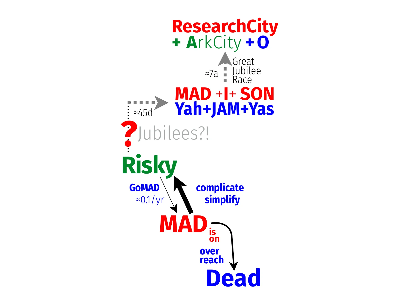
Figure 1: The RiskyMAD/MADI decision overview. Three states, four transitions. The escape path (Risky → LifeMAP) is currently inactive (rate = 0). Source: SD1.#
Risky — the current state of global affairs. Nuclear weapons exist, are deployed, and are on various levels of alert. No nuclear exchange has occurred. The system is metastable: it appears stable but has a non-zero probability per unit time of transitioning to the next state.
MAD — a crisis state in which nuclear exchange becomes imminent. This state is transient: the system either escalates to Dead or de-escalates back to Risky. The average crisis duration in the model is approximately 40 days (consistent with historical crises such as the Cuban Missile Crisis, which lasted 13 days).
Dead — accidental nuclear winter has been initiated. This state is absorbing: once entered, it cannot be left. The consequences of even a “limited” nuclear exchange (100+ warheads) include global temperature drops of 5–10 °C, agricultural collapse, and famine affecting billions. The state is named “Dead” not because every human dies, but because the civilization that produced nuclear weapons has entered irreversible collapse. Limited nuclear exchanges that do not trigger global winter are not modeled as “Dead” — they register only as milestones on the path to normalizing nuclear weapons enough that a global exchange becomes thinkable enough to happen.
The four transitions are:
Risky |rarr| MAD (rate:
rRiskyGoMAD= 0.10/year): a crisis arises that brings the system to the nuclear brink.MAD |rarr| Risky (rate:
rMADescapes= 6/year): the crisis de-escalates without nuclear exchange.MAD |rarr| Dead (rate:
rMADtoDEATH= 3/year): the crisis escalates to nuclear exchange and accidental nuclear winter.Risky |rarr| LifeMAP (rate:
rRiskyEscape= 0): the civilization transitions to Mutually Assured Progress. This transition is the escape — but in the base model, the rate is zero (no escape mechanism is currently active).
2.2 The Death-Trifecta Parameter: Why 1/3#
When the system enters a crisis (MAD state), two competing processes race: de-escalation (rate 6) and escalation to nuclear exchange (rate 3). The probability of death per crisis is therefore 3/(6+3) = 1/3.
This parameter is not arbitrary. It is grounded in the OSCR mechanism — a systems-failure pattern formally derived in Matheo-b12 (BABL definition and m6.th1, the OSCR Collapse theorem).
BABL (Blindly Assuming Blind Leveraging) is a systems-failure pattern that operates through three modes called the OSCR mechanism: over-Simplifying (reducing a complex problem to a false narrative), over-Complicating (burying the problem under layers of work-arounds), and over-Reaching (extending beyond the point of no return). This death-trifecta can be shown to invade any complex system, functioning like a zero-day exploit: it produces the same failure modes regardless of the system’s specific domain. For the formal derivation, see Matheo-b12.
Under BABL, a crisis resolves through one of three OSCR modes:
Over-Simplifying — the crisis is reduced to a manageable narrative (“it was just a misunderstanding”), and the system returns to Risky. The underlying tensions are unresolved, merely deferred.
Over-Complicating — the crisis generates layers of diplomatic work-arounds, and the system returns to Risky. The underlying tensions are buried under complexity, merely deferred.
Over-Reaching — someone, either by accident, by deliberate action, or by not realizing the implications of their orders, reaches beyond the point of no return. The RED button is pressed. Nuclear exchange begins.
Two out of three OSCR modes produce temporary escape (back to Risky).
One out of three produces death. Hence: rMADescapes = 6 (two
escape modes, each at rate 3) and rMADtoDEATH = 3 (one death mode
at rate 3). The factor of 3 sets the crisis time scale.
The equiprobability of the three OSCR modes is a modeling assumption, not a derived result. The three-mode structure is a structural property of BABL systems (formally derived in Matheo-b12, BABL definition and m6.th1); the equal weighting of the three modes is a simplifying choice. The sensitivity analysis in Section 2.5a shows that the qualitative conclusion does not depend on this choice.
The only empirical anchor, and it is a weak one. President Kennedy, in a private assessment to his Special Counsel Theodore Sorensen during the Cuban Missile Crisis, estimated the probability of nuclear war “somewhere between one in three, and even” (Sorensen, Kennedy, Harper & Row, 1965; confirmed in Sorensen’s 1986 WGBH interview for War and Peace in the Nuclear Age; widely cited via Allison and Zelikow, Essence of Decision, 2nd ed., Longman, 1999). This is the closest thing to a measurement of \(p_{death}\) that exists: one crisis participant’s subjective estimate, from inside one crisis, recorded second-hand. It is a single data point and it does not corroborate the parameter. It brackets it.
And the bracket runs both ways, which is the honest way to state this. Against Kennedy’s range of 1/3 to 1/2, the model’s 1/3 is the low end — his midpoint would be roughly 5/12, and using it would raise every figure in this paper by a quarter. Against the historical record read through Laplace’s rule (Section 2.8), the model’s 1/3 is roughly 3.7x too high at \(n = 4\). So the two available anchors pull in opposite directions and the chosen value sits between them, closer to the one that produces the lower forecast of the two. The parameter is not measured. It is bracketed by a subjective recollection on one side and an estimator with known defects on the other, and the paper says so rather than picking the flattering anchor and calling it support.
The precise value does not determine the conclusion. The model’s parameters can be tuned by adjusting the thresholds: what qualifies as a “nuclear MAD crisis” and what qualifies as “Dead.” The qualitative conclusion — stochastic certainty of accidental nuclear winter in the absence of structural change — holds across a wide range of parameter values (see Sections 2.5 and 2.5a).
2.3 Calibrating the Crisis Rate#
The critical parameter is \(\lambda\) (rRiskyGoMAD) — the rate at which
civilization-threatening nuclear crises arise. Everything else in the forecast is either
structural (Section 2.2) or algebra (Section 2.4a); this is the one number that must come
from the world.
The criterion. A civilization-threatening nuclear crisis — an entry into the MAD state — is any incident in which at least one nuclear-armed party’s command authority was confronted with a launch/no-launch decision, or in which nuclear weapons were physically brought to the brink of detonation. This criterion was fixed before counting and is applied unchanged below. That order matters: a criterion adjusted after seeing the count is not a measurement.
The source. Rather than assemble a private list, this paper calibrates against the largest published catalogue: the 60 historical incidents compiled by Baum, de Neufville and Barrett (2018) [Baum et al., 2018]. Using someone else’s data removes one degree of freedom from an exercise that has too many. The classification below is this paper’s own and is the part a reader should attack first; the underlying incidents are not.
Incidents are not excursions. This distinction does most of the work and is easy to miss. Six of Baum et al.’s sixty entries belong to the same Cuban missile crisis: the crisis itself, the Duluth–Volk bear incident, the B-59 submarine, the Okinawa missile order, the Florida satellite false alarm, and the Penkovsky false warning. The parameter \(\lambda\) counts entries into the MAD state, not incidents, so those six contribute one. Lewis et al. (2014) [Lewis et al., 2014] independently list four separate Cuban-crisis entries, which corroborates the distinction from outside this paper. A catalogue of sixty incidents therefore does not imply sixty crises, and any calibration that treats it as one will overstate \(\lambda\) by roughly an order of magnitude.
What the classification returns. Of the sixty incidents, twenty-seven are excluded as peripheral — nuclear threat rhetoric, contingency studies, failed acquisition attempts by non-state actors, and weapons accidents with no live launch pathway. A further twenty-three are serious but were caught by procedure rather than by human judgment or luck; these are the subject of Table 2. The remainder, after collapsing the Cuban-crisis entries, are the five excursions of Table 1 — of which four fall inside the forty Cold-War years, giving
On the composition of “the four”. Published and popular lists of the most widely acknowledged near-misses do not agree on membership: this paper’s reconstruction, the lists circulating in popular accounts, and Lewis et al.’s Table 1 select different events. That disagreement is real and is the subject of Table 2. It does not make the count worthless. Four Cuba-grade excursions in the forty Cold-War years is what this reconstruction returns from someone else’s dataset, under a criterion fixed in advance — and an independent expert count, obtained by personal communication and by a different route, returns the same number.
# |
Year |
Event |
Explanation — what actually happened |
Why it qualifies |
Cold War? |
|---|---|---|---|---|---|
1 |
1961 |
Berlin Crisis [c] |
The USSR demanded Western forces leave West Berlin. In October, Kennedy considered a first strike: a White House/Pentagon group produced a detailed plan to destroy Soviet second-strike capability by attacking 1,077 targets, after intelligence showed a much larger US arsenal than believed. He gave a speech instead. |
a disarming first-strike plan reached the President’s desk |
yes |
2 |
1962 |
Cuban Missile Crisis |
The reference event. Thirteen days. Internally it contains at least five further incidents (see note below), including the B-59 submarine, whose captain ordered the nuclear torpedo prepared and was overruled by Vasili Arkhipov. |
launch decisions reached officers with authority; refusal, not procedure, stopped them |
yes |
3 |
1983 |
Petrov (Serpukhov-15) [a] |
Soviet satellites indicated an incoming US missile launch. Duty officer Stanislav Petrov judged it a false alarm and declined to report it. He was right: sunlight on high cloud. |
a launch indication reached a human whose judgment was the filter |
yes |
4 |
1983 |
Able Archer |
A realistic NATO command exercise simulating nuclear release, during a period when Soviet leadership feared a genuine first strike. Soviet leadership moved to bunkers; nuclear bombers went to runway alert. |
Baum: “how close they were to launching their own attack is unclear” |
yes |
5 |
1995 |
Norwegian Rocket |
A Norwegian scientific rocket matched the flight profile of a submarine-launched missile intended to blind Russian radar by EMP. Russian forces went to full alert and Yeltsin activated the nuclear command suitcase — the only confirmed activation. |
launch authority was physically engaged by a head of state |
no |
– |
1945 |
World War II [b] |
The atomic bombings of Hiroshima and Nagasaki: the only historical instance of nuclear war. |
excluded from the rate — see [b] |
– |
Petrov — retained, with the reservation recorded. On Baum’s text alone, roughly five missiles were indicated, which is implausible for a first strike, and downstream corroboration would very likely have failed; on a strict reading the decision never reached release authority. He is retained because he is among the most widely acknowledged near-misses and because Lewis et al. (2014) independently include him (Serpukhov-15, Table 1). The forecast does not depend on him: excluding Petrov gives three Cold-War excursions, a crisis rate of 0.075/yr, and an annual onset probability of 2.19 percent — 1 in 46.
World War II — excluded from the rate, and why it is nonetheless in the table. It was a one-sided use, not an entry into the two-sided crisis state this model tracks, so it is not an observation of \(\lambda\). What it establishes is not a probability but a capability: that these weapons were in fact deployed against whatever objections stood in the way at the time. The model assumes \(c > 0\). World War II is the observation that \(c > 0\) is not a hypothesis.
Berlin 1961 is this paper’s own addition and is not in Lewis et al.’s list. It is included because a live disarming-first-strike plan reaching a head of state meets the criterion in Section 2.3 more directly than several incidents that are conventionally listed. A reader who rejects it should use the three-excursion row above.
How many incidents count as near nuclear use is contested in the published literature, and Baum names the dispute: “analysts disagree on how close they were to nuclear war — for example, Lewis et al. (2014) consider them to have come pretty close, while Tertrais (2017) disagrees.” Rather than adjudicate it, this paper reports both poles and shows what each implies.
Position |
Count |
Explanation — what they counted |
\(\lambda\) (/yr) |
P(onset ≤ 1 yr) |
|---|---|---|---|---|
Tertrais (2017), skeptical |
1 |
37 episodes reviewed; concludes safety mechanisms held throughout, and that only one significant incident has occurred in ~34 years (Black Brant, 1995). Excludes accidents, unauthorized launch, and terrorism by stated scope. |
0.029 |
0.85% (1 in 117) |
This paper, Table 1 |
4 (Cold War) |
Berlin 1961, Cuba 1962, Petrov 1983, Able Archer 1983; criteria fixed before counting; Norwegian Rocket 1995 falls outside the Cold-War window. |
0.100 |
2.90% (1 in 34) |
Lewis et al. (2014), inclusive |
6 (Cold War) |
Their Table 1 lists 13 cases of near nuclear use; collapsed to excursions (four of the thirteen are Cuban-crisis entries) this gives six Cold-War excursions: Cuba 1962, the 1973 Arab–Israeli war, NORAD 1979, NORAD 1980, Serpukhov-15 1983, Able Archer 1983. |
0.150 |
4.30% (1 in 23) |
Lewis et al., whole era |
10 / 77 yr |
Adds the 1991 Soviet coup, Black Brant 1995, Kargil 1999, and the 2001–02 Kashmir standoff. |
0.130 |
3.75% (1 in 27) |
Three things follow, and the second is the one that matters.
The scenario range of Section 2.5 contains both published poles. The optimistic corner (0.03/yr) is Tertrais’s implied rate. The pessimistic corner (0.3/yr) lies above Lewis et al.’s — it is not supported by either pole and rests instead on the non-stationarity argument of Section 2.10, where it is argued rather than cited.
This paper’s base case is more conservative than Chatham House. Lewis et al.’s reading implies 1 in 23 per year; the base case used here is 1 in 34. A paper that adopted the most inclusive published position wholesale would forecast a higher risk than this one does. Whatever else this forecast is, it is not the most alarming reading available in the literature.
The disagreement is narrower than it looks. The two poles are separated by a factor of about five in \(\lambda\) — and, because the anchor of Section 2.0a is robust across that whole span, they are not separated at all on the question the paper actually asks. See Table 3.
2.4 The Model Code and Simulation Results#
The RiskyMAD model was implemented in the Evolvix prototype compiler (MMv0r3p1-RC1) and run as a stochastic simulation using the Gillespie algorithm (Gillespie, 1977) — the standard method for exact stochastic simulation of continuous-time Markov chains.
The complete model code (as published on the SD1 poster):
Evolvix Quest RiskyMADdead
(Question: "How many years until humanity self-destructs
            in a nuclear roulette accident?")

Simulate stochastically until 200 :["years"]

Initial Amount of Risky       = 1
Initial Amount of MAD         = 0
Initial Amount of Dead        = 0
Initial Amount of rRiskyGoMAD = 0.10
Initial Amount of rMADescapes = 6
Initial Amount of rMADtoDEATH = 3

Action 1 ( Risky ---[ Rate = 0.10 ]---> MAD     )
Action 2 ( MAD   ---[ Rate = 6    ]---> Risky   )
Action 3 ( MAD   ---[ Rate = 3    ]---> Dead    )
Action 4 ( Risky ---[ Rate = 0    ]---> LifeMAP )
This is the entire model. In other simulation frameworks, implementing a continuous-time Markov chain with Gillespie dynamics requires hundreds of lines of code. In Evolvix, the model fits on a poster. Anyone who can read the code can check the math. The Evolvix prototype compiler is available for download at Evolvix Prototype Compiler — Download and RiskyMAD Model Code.
Simulation results (40 independent stochastic runs per scenario):
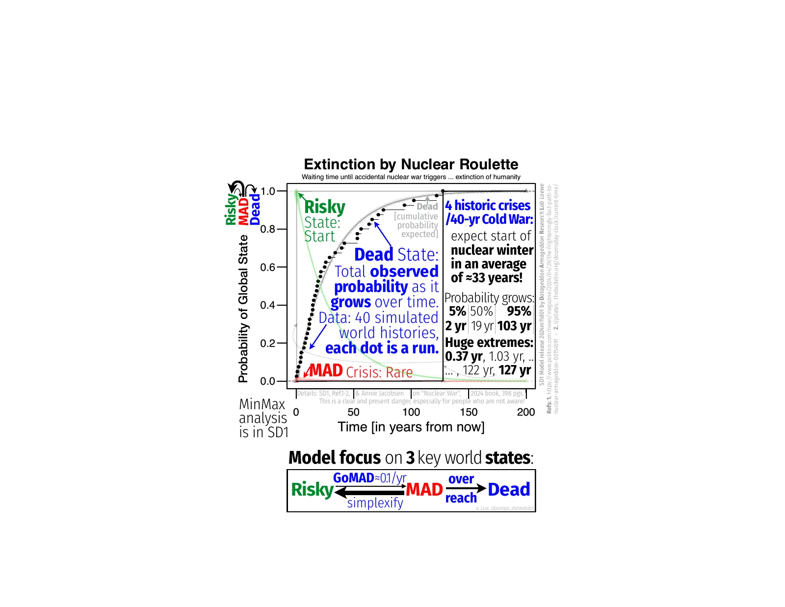
Figure 2: Stochastic inevitability of accidental nuclear winter. Forty simulation runs for each parameter scenario. In the most optimistic scenario, the luckiest runs reach ~329 years. In the most pessimistic, the fastest runs produce accidental nuclear winter within days. The argument holds equally whether the waiting time is 4 days or 3 centuries. Source: SD1.#
Scenario |
|
Median |
Mean |
Min |
Max |
Key finding |
|---|---|---|---|---|---|---|
Pessimistic |
0.3/year |
~6.4 yr |
~10 yr |
0.01 yr |
36 yr |
Fastest runs: accidental nuclear winter within days |
Base |
0.1/year |
~19 yr |
~33 yr |
0.37 yr |
127 yr |
Accidental nuclear winter within a generation |
Optimistic |
0.03/year |
~51 yr |
~96 yr |
0.57 yr |
329 yr |
Luckiest runs reach ~329 years; median still within a lifetime |
2.4a Analytic Solution: Mean Time to Absorption#
The simulation is not the only handle on this model. The chain is small enough to solve exactly, and doing so both supplies the waiting times this paper reports and retires a standing objection.
Let \(T_R\) and \(T_M\) be the expected times to reach Dead from Risky and from MAD. Conditioning on the next transition:
Solving the pair:
At the base crisis rate of 0.1/yr, with \(b = 6\) and \(c = 3\): \(T_R = 9/0.3 + 1/3 = 30.3\) years.
But the mean is not the distribution, and the difference matters at short horizons. Reporting \(P(\text{onset} \le t)\) requires the whole first-passage law, not its average. Taking the Laplace transform of the same conditioning argument, with \(f_R(s) = \mathbb{E}[e^{-sT_R}]\):
The denominator factorises as \((s+r_1)(s+r_2)\) with \(r_1 r_2 = \lambda c\) and \(r_1 + r_2 = \lambda + b + c\). Since the transform is exactly \(r_1 r_2 / [(s+r_1)(s+r_2)]\), the waiting time is hypoexponential — the sum of two independent exponentials, not one:
At the base rate: \(r_1 = 0.0331\)/yr (the onset hazard — the slow stage, the wait for a crisis to arrive and escalate) and \(r_2 = 9.067\)/yr (the fast stage, the crisis itself, mean duration 40 days). Every figure in Table 3 comes from this expression.
Why this matters only at one year, and why it matters there. The fast stage contributes a mean delay of about forty days before onset is even possible, which suppresses the distribution near the origin. Over ten years or more the suppression is negligible and an exponential fitted to \(T_R\) agrees to within 0.2 percentage points — which is why the longer columns of Table 3 barely moved. At one year the forty days are 11 percent of the window, and the exponential shortcut overstates the answer by ~12 percent in every scenario: 3.24% against the true 2.90% at base. The one-year figure is the one everybody quotes. The shortcut erred there, and it erred upward.
The structure answers the “loop” objection. It is sometimes put to this model that the de-escalation path MAD \(\rightarrow\) Risky \(\rightarrow\) MAD gives the world repeated chances to survive, and that a forecast ignoring those chances must overstate the risk. The objection is reasonable and the mathematics has already answered it. The factor
The structure is interpretable, and it answers the “loop” objection. It is sometimes put to this model that the de-escalation path MAD \(\rightarrow\) Risky \(\rightarrow\) MAD gives the world repeated chances to survive, and that a forecast which ignores those chances must overstate the risk. The objection is reasonable and the mathematics has already answered it. The factor
is exactly the expected number of excursions into MAD before one escalates — a geometric process with per-crisis death probability \(p_{death} = c/(b+c) = 1/3\), hence a mean of three attempts. Each attempt is preceded by an average wait of \(1/\lambda = 10\) years in Risky. So \(T_R \approx 3 \times 10\) years. The de-escalation loop is not omitted from the mathematics: it is the factor of three. The world does get another chance, and the model counts every one of them.
The Poisson form is checked, and it holds — as a rate. The onset hazard from the exact solution is \(r_1 = 0.0331\)/yr; the Poisson rate \(\lambda \cdot p_{death} = 0.0333\)/yr. They agree to within 1 percent, because time spent inside a crisis slightly delays the onset of the next one. What does not follow is that either rate may be fed into \(1 - \exp(-rt)\) to obtain a one-year probability. That is the step the hypoexponential form above forbids: a rate is not a distribution when the process has two stages and the horizon is comparable to the short one. The agreement of the rates is real; the shortcut it appears to license is not.
2.5 Worst, Mid and Best: Running World History Forward#
Central Result
At the base crisis rate, half of all runs of world history reach accidental nuclear winter within 21 years. The annual probability that it begins is 2.90 percent — about 1 in 34 — and across the full scenario range it lies between roughly 1 percent and 8 percent. That range is a bound, and the bound is the result.
The simulation findings hold. The arithmetic sharpens them. Forty independent runs of world history returned a median near 19 years, and roughly one run in forty reached catastrophe inside the first year. Solving the model exactly (Section 2.4a) puts the median at 21.1 years and predicts 1.16 blow-ups per forty runs. Both simulated figures sit within ordinary sampling noise of the exact ones. Nothing here overturns what the simulations showed; it measures the same thing with a finer instrument, and the finer instrument reads slightly worse, not better.
The paper’s earlier “at least 1 in 40” formulation was close, and errs in one place only. As a floor on the annual probability it holds at the base rate (2.90 percent) and in the pessimistic scenario (8.34 percent). It over-states the risk at the optimistic corner, where the exact value is 0.88 percent — 1 in 113. That is the honest correction: the formulation was right where it mattered and too pessimistic at the best-case end.
One claim does not survive, and it should never have been made: that 1-in-40 held regardless of scenario. It does not. The expected number of blow-ups per forty runs is 0.35 optimistic, 1.16 base, 3.34 pessimistic — a spread of nearly ten. A uniform 1-in-40 was never a result of this model; it was a tidy-looking summary that a hedged statement collapsed into somewhere between the simulations and the prose, and it is removed here rather than defended.
Two instruments, two jobs. This section reports simulations and arithmetic, and they are not doing the same work, and keeping them apart is what makes each of them useful.
The simulations run world history forward and return waiting times. They are the right instrument for the shape of the distribution — the medians, the long tails, the fact that some runs last a century. That shape is what Section 2.7 rests on.
The arithmetic returns the annual probability. It is exact and closed-form. Forty runs cannot resolve a 3 percent probability — the standard error on such an estimate at \(n = 40\) is about 2.5 percent, which is nearly the estimate itself — so the simulations are simply the wrong tool for that number, and no re-run would change this.
They agree, and the agreement is now reportable rather than hedged: see below.
What was simulated. Forty independent runs of world history per scenario, generated with the Evolvix prototype compiler (download), which implements the stochastic simulation algorithm exactly (Gillespie, 1977; Ehlert & Loewe, 2014, “Lazy Updating,” J Chem Phys 141(20): 204109). Each run produces one random waiting time until accidental nuclear winter.
Figure 2: Forty runs of world history for each scenario — optimistic, base, and pessimistic. In the most optimistic, the luckiest run reaches ~329 years. In the most pessimistic, the fastest runs produce accidental nuclear winter within days. The argument holds equally whether the waiting time is four days or three centuries — which is the point of showing all three. Source: SD1.#
Scenario |
crisis rate |
median |
mean |
fastest run |
slowest run |
What the runs show |
|---|---|---|---|---|---|---|
Optimistic |
0.03/yr |
~51 yr |
~96 yr |
0.57 yr |
329 yr |
Luckiest run reaches three centuries; median still inside one lifetime |
Base |
0.10/yr |
~19 yr |
~33 yr |
0.37 yr |
127 yr |
Onset within a generation, with a century-long tail |
Pessimistic |
0.30/yr |
~6.4 yr |
~10 yr |
0.01 yr |
36 yr |
Fastest runs produce accidental nuclear winter within days |
Scenario |
crisis rate |
mean |
median |
≤ 1 yr |
≤ 10 yr |
≤ 20 yr |
≤ 40 yr |
|---|---|---|---|---|---|---|---|
optimistic (= Tertrais) |
0.03 |
100.3 yr |
69.6 yr |
0.88% |
9.40% |
18.00% |
32.83% |
base |
0.10 |
30.3 yr |
21.1 yr |
2.90% |
27.91% |
48.22% |
73.28% |
(= Lewis et al.) |
0.15 |
20.3 yr |
14.1 yr |
4.30% |
38.68% |
62.60% |
86.09% |
Petrov removed (§7.1b) |
0.075 |
40.3 yr |
28.0 yr |
2.19% |
21.8% |
39.0% |
62.9% |
pessimistic |
0.30 |
10.3 yr |
7.2 yr |
8.34% |
61.99% |
85.71% |
97.98% |
The two tables agree, and the agreement is checkable. At the base rate the exact one-year probability is 2.90 percent, so the expected number of the forty runs that blow up inside the first year is \(40 \times 0.0290 = 1.16\). Observing one or two such runs is the ordinary outcome — \(P(X \ge 2) = 32\) percent. The simulated medians sit below the exact ones (~19 against 21.1 at base) by an amount that is unremarkable at \(n=40\). There is no tension between the two instruments, and the appearance of one in earlier drafts was manufactured by the exponential shortcut the previous section retired: it inflated the arithmetic to 3.24 percent and left the simulations looking as though they disagreed. They never did.
On the 127-year run. The slowest of the forty base-case runs reached 127 years. That is an observed sample maximum, not a probability: the exact chance of exceeding 127 years at the base rate is 1.50 percent, or about 1 in 67, and the expected maximum of forty draws falls near 112 years. “Roughly one run in forty survives past 127 years” would read as a distributional claim and is not one. The run is quoted here only for what it shows: that this model produces century-long quiet stretches as a matter of course (Section 2.7).
What a 1-in-34 annual probability means. No regulator, no underwriter, and no operator of any other system accepts a 3 percent annual chance of catastrophic, irreversible failure. This one is accepted — not through informed consent, and not because anyone weighed it and judged it tolerable, but because almost nobody has been shown the number. Section 2.6 puts it beside a risk that societies have weighed and do accept. .. _oov1-b16-sec2-5a:
2.5a Sensitivity Analysis: Death Probability#
The base model uses a per-crisis death probability of 1/3, grounded in the OSCR three-mode structure (Section 2.2). The equiprobability of the three modes is a modelling assumption, and Section 7.3 states plainly that it is the weakest joint in this paper. This table shows what happens when it is varied, holding the crisis rate at its base value of 0.1/yr.
per-crisis death prob. |
implied rates |
mean |
median |
P(onset ≤ 1 yr) |
x car-crash |
|---|---|---|---|---|---|
1/10 |
|
100.3 yr |
69.6 yr |
0.96% |
19x |
1/5 |
|
50.3 yr |
34.9 yr |
1.84% |
37x |
1/3 (base case) |
|
30.3 yr |
21.1 yr |
2.90% |
58x |
1/2 (= Kennedy’s upper end) |
|
20.3 yr |
14.1 yr |
4.05% |
82x |
These are exact values. A 40-run sample would put the base-case median near 19 years against the exact 21.1, and the 1/10 row near 57 against 69.6 — ordinary noise, but there is no reason to quote a noisy sample when a closed form exists (Section 2.5). Every figure above comes from the first-passage law of Section 2.4a. The car-crash column uses the global baseline and \(q = 0.3\) (Section 2.6).
The parameter moves the waiting time, not the direction. Across the whole range — from a tenth to a half, which spans every value anyone has proposed, including both ends of Kennedy’s estimate — the mean wait moves by a factor of five and the car-crash comparison never falls below 19x. Even at 1/10, a value below anything this paper’s structure or its anecdotal anchor suggests, an individual remains an order of magnitude more likely to die of accidental nuclear winter than in a car crash.
And stochastic certainty holds for any death probability above zero. Whether the value is 1/10 or 1/2, the absorbing state is reached with probability 1 given sufficient time (Section 2.9). The parameter sets the schedule. It does not set the outcome.
2.6 Contextualizing the Risk: The Car-Crash Baseline#
To make the forecast tangible, it is compared against a mortality risk that societies accept without alarm: dying in a motor-vehicle crash. The comparison must be like-for-like — annual probability, per person, death against death — or it is meaningless. Three quantities are therefore kept distinct throughout.
The baseline. Worldwide, road traffic kills about 1.19 million people a year, a rate of roughly 15 per 100,000 population, or \(1.49\times10^{-4}\) per person per year — about 1 in 6,700 [World Health Organization, 2023]. This paper uses the global figure, because its claim is about most people. The United States rate (\(1.22\times10^{-4}\); 40,901 deaths at 12.21 per 100,000 in 2023 [National Highway Traffic Safety Administration, 2024]) is lower than the global average, so using it would inflate every multiplier below — which is the direction a reader should expect a motivated author to choose, and the reason not to.
The model’s output is not a mortality. RiskyMAD forecasts the annual probability that accidental nuclear winter begins — not the probability that any given individual dies. The two differ by the death fraction
driven by global cooling, agricultural collapse, and famine. Individual annual mortality is therefore \(P(\text{onset}) \times q\), and it is this product — not \(P(\text{onset})\) — that may be set beside the road-death figure. Conflating the two would overstate the comparison by a factor of \(1/q\).
Where \(q\) comes from. It is not this model’s output and is not invented here. Xia et al. (2022) estimate that even a small regional exchange — roughly 100 warheads, 5 Tg of soot — causes about 2 billion deaths from famine within two years, while a full US–Russia exchange (150 Tg) causes over 5 billion [Xia et al., 2022]. Against a world population near 8 billion those are \(q \approx 0.25\) and \(q \approx 0.63\). This paper uses \(q = 0.3\), near the low end of that published range and corresponding to the smallest exchange anyone models.
Scenario |
P(onset ≤ 1 yr) |
Individual mortality |
Relative to road deaths |
|---|---|---|---|
optimistic (= Tertrais’s implied rate) |
0.88% |
\(2.6 \times 10^{-3}\) |
18x |
base |
2.90% |
\(8.7 \times 10^{-3}\) |
58x |
Lewis et al.’s implied rate |
4.30% |
\(1.3 \times 10^{-2}\) |
87x |
pessimistic |
8.34% |
\(2.5 \times 10^{-2}\) |
168x |
The stress test. Three inputs to that table are chosen rather than measured: the crisis rate, the death fraction, and the baseline. A reader is entitled to suspect that three choices all landing in the paper’s favour is not a coincidence. So each is pushed to its least favourable defensible value at the same time:
Input |
Least favourable defensible value |
Why that value is admissible |
|---|---|---|
crisis rate |
0.03/yr (P = 0.88%) |
Tertrais’s own reading of the record — the most sceptical published position (Section 5.3) |
death fraction \(q\) |
0.25 |
Xia et al.’s smallest modelled exchange, 100 warheads [Xia et al., 2022] |
baseline |
7.3e-4/yr |
Libya, ~73.4 per 100,000 (2013) — the highest national rate on record, nearly five times the global average [World Health Organization, 2015] [Guinness World Records, 2013] |
What survives the stress test
Against the global baseline, with the most sceptical crisis rate and the lowest published death fraction: 15x.
Against the road-death rate of the worst-affected country on record — Libya, at nearly five times the global average — with those same two concessions: 3x.
The inequality holds at every corner, including all three corners at once. It is not rescued by any single input, and it cannot be attacked by disputing any single input. That is the claim this paper defends. The multiplier is a range — roughly threefold at the most punishing corner constructible, sixtyfold at the base case, a few hundredfold at the pessimistic one. The direction does not move.
On the worst-country figure. The baseline used here is the highest national road-death rate on record — Libya at 73.4 per 100,000 in 2013, reported in WHO’s Global status report on road safety 2015 [World Health Organization, 2015] and recorded by Guinness World Records as the world’s deadliest place to travel by road [Guinness World Records, 2013]. It is chosen deliberately as the most demanding baseline the record supports: a higher road-death rate makes the car-crash comparison harder, so surviving against it is the strongest form of the claim. Libya’s more recent WHO figure is lower (~34 per 100,000, 2021 [World Health Organization, 2023]), and national rankings shift year to year — nothing here turns on Libya being worst today, only on 73.4 being a real, documented maximum. At the current ~34 the multiplier would be larger (about 6.5x rather than 3x), so this choice is the conservative one.
The scope switch, and why the number of billions does not matter. Individual annual mortality is the only axis on which these two risks are commensurable, which is why the comparison runs there. On every other axis they differ, and every difference runs the same way. A car crash is idiosyncratic: it kills you and perhaps a few others; the world continues; an insurer pays; your family is compensated; the institutions that investigate the crash still exist the next morning. Nuclear winter is systemic: it kills you, and everyone you know, and the institutions, and the counterparty, and the investigator.
This is why nothing in the argument depends on whether the toll is one billion or eight. At \(q = 0.25\) the inequality holds; at \(q = 1\) it holds; only the multiplier moves. And the character of the risk — perfectly correlated across the whole population, with no surviving counterparty — is identical at every \(q > 0\). A reader who wants to argue about the billions is arguing about a number the conclusion does not use.
The risk is not unpriced. It was priced, and the price was “uninsurable.”
It is tempting to call this risk “uninsured, unregulated, unpriced”, as though through oversight. That would be wrong, and the truth is stronger.
Nuclear war is excluded from essentially every insurance policy written — property, casualty, life — by a standard nuclear exclusion clause [U.S. Government Accountability Office, 2008]. Not because the risk is small. Because it is uninsurable in principle: insurance requires risks that are independent, so that a pool can absorb them, and a solvent counterparty who survives to pay. Nuclear winter violates both, by construction. The United States Treasury told Congress as much: war insurance “is not a feasible means for handling war losses of the magnitude which might be expected in a nuclear conflict.”
So the profession that prices catastrophic risk for a living has already examined this one and declined it. That is not ignorance — it is a decision, taken decades ago, and documented in the fine print of nearly every policy on Earth. The risk is not unpriced. It is priced at infinity, and then not spoken of again.
The inequality in Table 6 is therefore not a claim that actuaries have missed something. It is a claim about what happens when a risk is removed from the domain where risk expertise operates: it stops being measured, and then it stops being mentioned, and then people conclude from the silence that it is small.
The pattern is visible in the government’s own record. When the United States asked whether nuclear, biological, chemical and radiological attacks were insurable, the resulting review [U.S. Government Accountability Office, 2008] catalogued the exclusions and the potential for catastrophic loss — the severity side — but did not estimate how likely such an event is; frequency was treated as outside the question. Set that beside an age that funds sky-surveys to put numbers on asteroid-impact probabilities: for nuclear war the risk apparatus returns a severity verdict, “uninsurable,” and leaves the likelihood unasked. That unasked question — how often — is the one this study answers.
Note
On the distinction between the exchange and the winter. A nuclear exchange between two states might kill millions directly. The subsequent nuclear winter — global cooling, agricultural collapse, famine — is what kills billions. The winter, not the exchange, is the mass killer, which is why the model treats nuclear winter as the absorbing state rather than weapon launch. This also means the estimate here is not comparable to forecasts whose terminal event is a launch (Section 5.2): the states being forecast are different, and the difference runs in the direction of a broader, later, and more consequential threshold.
Caution
:math:`q` is the softest number in this paper, and it is doing real work. Every figure in Table 6 scales linearly with it. It is anchored to Xia et al. [Xia et al., 2022] rather than derived here, and the anchoring is coarse: their scenarios are specific exchanges, and this model’s absorbing state is not resolved to a warhead count. A reader who prefers a different \(q\) may rescale Table 6’s final column directly. The inequality against the global baseline survives for any \(q > 0.017\) — computed at the optimistic corner, which is the one this paper leans on, and roughly fifteen times below the lowest published estimate. Note that the threshold must be computed at that corner: taken at the base case it would read \(q > 0.004\), which does not hold where the paper actually leans.
2.7 The Mechanism: Michaelis–Menten Kinetics#
The preceding sections produce a number. This section gives the reason the number has the shape it does. It earns its space because the mechanism answers an objection that no amount of arithmetic can reach: nothing has happened in eighty years, so how bad can it be?
The claim, stated precisely. The scheme Risky \(\rightleftharpoons\) MAD \(\rightarrow\) Dead is not merely reminiscent of enzyme kinetics. Solving its own first-passage equations (Section 2.4a) for the rate at which the chain reaches Dead gives
which is identical, at every point, to the Michaelis–Menten rate law
under the reading below. This is not an analogy that holds approximately in a limit. It is the same function.
Michaelis–Menten |
RiskyMAD |
Value |
Meaning here |
|---|---|---|---|
substrate \(S\) |
crisis rate \(\lambda\) |
0.1/yr |
how often the world enters a nuclear crisis |
\(K_m\) |
\(b + c\) |
9/yr |
how fast a crisis resolves, either way |
\(V_{max}\) |
\(c\) |
3/yr |
the escalation step — you cannot die faster than this |
\(k_{cat}/K_m\) |
\(V_{max}/K_m = c/(b+c)\) |
1/3 |
the specificity constant |
commitment to catalysis |
\(p_{death} = c/(b+c)\) |
1/3 |
the fraction of crises that go all the way |
The defining property of Michaelis–Menten kinetics holds exactly: the rate is half-maximal when \(S = K_m\). Here \(v(9) = 1.5 = V_{max}/2\). And the system saturates: as \(\lambda \rightarrow \infty\), \(v \rightarrow c\). That ceiling is not a mathematical curiosity — it says that however often crises arrive, the world cannot be destroyed faster than the escalation step permits.
Why “but the master equations are linear” is not an objection. It has been put to the authors that this model cannot be Michaelis–Menten because there is no substrate concentration, no conserved catalyst, and because the governing master equations are linear. The premise is true and the conclusion does not follow.
Single-molecule Michaelis–Menten kinetics — one enzyme, one substrate, first passage to one product — also has linear master equations. That is what makes it tractable, and it is a developed field in its own right. The linearity is in the state probabilities; the saturation is in the \(\lambda\)-dependence of the first-passage rate. Both are true at once, in this model and in real enzymology, and neither implies the other. There is likewise no requirement for a concentration: in the count-based reading, \(S\) is an encounter rate, not a concentration, and the dimensionless ratio \(\lambda/(b+c)\) does the work that \([S]/K_m\) does in the textbook treatment. This model has one Earth and one doomsday system, and that is exactly the regime single-molecule kinetics was built for.
Why the analogy earns its keep. The value of Michaelis–Menten kinetics has never been that enzymes are simple. They are not: an enzyme is a large machine that wanders through an enormous configuration space, and the details of how it finds and binds its substrate are, in the general case, hopeless to model. The achievement of the Michaelis–Menten treatment is that you do not need them. All of that unmodellable complexity is absorbed into an effective encounter rate, and the waiting time to product follows from that rate and two others.
The same structure holds here, and it is the reason this paper can exist. The “configuration space” is the space of historical causal chains — every way the world can arrange itself into a nuclear crisis. No one can model that. But it is not necessary to model it, because the encounter rate can be measured instead, from the record of times the world did in fact enter such a state. That measurement is Section 2.3, and Tables 1 and 2 are what it returns. The near-miss record plays exactly the role that a measured \(k_{on}[S]\) plays in enzymology: it is the empirical stand-in for a mechanism too complex to derive.
Where this system actually sits. With \(\lambda = 0.1\)/yr and \(K_m = 9\)/yr, the ratio is
— ninety times below half-saturation. The system is deep in the first-order regime, and this is why the simple product \(\lambda \cdot p_{death}\) works at all: it is the low-substrate limit of a saturating law, and it agrees with the exact solution to 1.1 percent. Saturation would require a crisis roughly every six weeks. The model is therefore operating in the regime where the analogy is not merely valid but linear — which is the easy case, and the one most favourable to a sceptical reader.
A consistency check that was not fitted. The parameters \(b\) and \(c\) were set from the OSCR structure (Section 2.2), with no reference to crisis durations. Yet they imply that a crisis, once entered, resolves in a mean time of \(1/(b+c) \approx 40\) days. The Cuban missile crisis lasted thirteen days. Those agree to well within an order of magnitude, from a parameter fixed for entirely independent reasons. This is offered not as confirmation but as the absence of a contradiction that could easily have appeared.
What the quiet years prove. The system spends about one percent of its time in the bound state: \(\lambda/(\lambda+b+c) \approx 0.011\). The rest of the time the doomsday substrate is elsewhere, and the world looks safe — because it is safe, most of the time. When binding occurs, the resolution is fast and the outcome is decided in weeks.
This is the shape of the risk, and it is why the intuition “nothing has happened, so the rate must be low” fails. A process that is quiescent 99 percent of the time and lethal 1/3 of the time it is not will produce long, calm stretches as a matter of course. In the base scenario the median wait to absorption is 21 years, yet roughly one run in forty survives past 127 years. Both are the same model. An observer inside the long run would conclude the risk was small; an observer inside the short one would not; and neither observation moves the underlying rate. The non-observation of nuclear war since 1945 is precisely what this model predicts most of the time, and it is therefore weak evidence about the parameters. That is not a rhetorical point. It is a property of the variance of first-passage times in a saturating two-step scheme, and it can be checked by running the model.
2.8 Alternative Re-weightings#
The scenario range of Section 2.5 takes \(p_{death} = 1/3\) from the OSCR structure and calibrates \(\lambda\) from the record. A reader may reasonably ask what happens if \(p_{death}\) is calibrated from the record too. This section reports that calculation, because a reviewer will perform it in ten minutes and it is better answered than ignored. It is presented as one analysis among several, and it is not the paper’s headline.
The calculation. Suppose \(n\) crises met the MAD criterion and none escalated. Under a uniform prior, the posterior mean of \(p\) is Laplace’s rule of succession, \(\mathbb{E}[p \mid 0 \text{ in } n] = 1/(n+2)\). Estimating \(\lambda = n/T\) from the same count over \(T = 77\) years gives an effective hazard
Counting more crises raises \(\lambda\) and lowers \(p\), and the two effects very nearly cancel: 0.86 percent per year at \(n=4\), 1.08 percent at \(n=10\), approaching 1.30 percent as \(n\) grows without bound. The limit \(1/T\) is what one obtains by discarding the crisis decomposition entirely and applying Laplace directly to the time axis. Notably, this converges on Hellman’s independently derived ~1 percent per year (Section 5.2) — two different routes, two different decades, the same order of magnitude.
Why this is reported and not adopted. Four reasons, and the first is the one that matters.
It is a re-weighting, not a measurement. Trading a rising \(\lambda\) against a falling \(p\) so that they cancel does not add information; it redistributes an assumption. The apparent stability of \(h_{\mathrm{eff}}\) across \(n\) is an artifact of the estimator’s construction, not a discovered invariance of the world.
\(1/T\) is a posterior mean under a flat prior, not a ceiling. It is frequently mistaken for one. The posterior on the hazard is wide, and it assigns non-negligible probability to values well above its own mean. Summarising an existential risk by the mean of a wide posterior is a false security illusion: it converts an unresolved question into a reassuring point estimate, which is precisely the failure mode this paper exists to name.
The record is weak evidence at \(n=4\). Surviving four crises each carrying \(p = 1/3\) has probability \((2/3)^4 = 19.8\) percent — unremarkable luck. The likelihood ratio between \(p = 1/3\) and \(p = 0.1\) is only about 3.3 to 1. A value derived from structure (Section 2.2) is not displaced by evidence that weak. The trade only bites for large \(n\), and Section 2.3 returns \(n = 4\).
At \(n = 1\) the rule returns \(p = 1/3\) exactly. If the Cuban missile crisis is treated as singular — which is what Hellman independently concludes when he reports that its thirteen days may carry more than a tenth of the era’s total risk — then Laplace and Kennedy agree to the digit. The disagreement between this section and Section 2.2 is therefore not about arithmetic. It is about whether Cuba was one of several comparable events or one of a kind.
The honest summary is that this re-weighting is an interesting convergence with the existing literature and a poor basis for a forecast. It is included so that a reader who reaches for it finds it already here, with its weaknesses stated.
2.9 Stochastic Certainty#
Note
This result is qualitative, and is not the forecast. The certainty result below is parameter-independent: it holds for any positive rates, and says only that an absorbing state is reached eventually. The quantitative annual probability is bounded in Section 2.5, and the waiting times in Section 2.4a. The two must not be read as one claim — certainty about the limit is not urgency about the year, and this paper’s case rests on Section 2.5, not on this section.
The most important structural insight is not the median (21 years) or the annual probability, but the mathematical certainty of the outcome:
As long as rRiskyGoMAD > 0 and rMADtoDEATH > 0,
accidental nuclear winter is a stochastic certainty. The absorbing
state (Dead) is reached with probability 1. Not probability 0.95.
Not probability 0.99. Probability 1. The only question is when.
The only way to change this conclusion is to make one of these parameters exactly zero — which means either eliminating nuclear crises entirely or ensuring that no crisis ever escalates to exchange. Neither is achievable without structural change to the system.
This is not a rhetorical claim. It is a theorem of absorbing Markov chains: any state that can be reached from any other state and that has no outgoing transitions will be reached with probability 1, given sufficient time. The Dead state is absorbing. It is reachable from Risky (via MAD). Therefore it will be reached. The parameters determine the waiting time, not the outcome.
The stochastic certainty result is timeline-independent. Whether the median waiting time is 4 days or 3 centuries, the conclusion is the same. The argument holds equally at every point in the full simulation range — from the fastest pessimistic runs (accidental nuclear winter within days) to the luckiest optimistic runs (~329 years). Those who claim the risk is manageable must demonstrate that the crisis rate reaches exactly zero — that no nuclear crisis will ever occur again. No credible analyst makes this claim.
2.10 Why the Crisis Rate Increases Over Time#
The base model assumes a constant crisis rate. This is a conservative simplification. The upstream papers provide formal reasons to expect the crisis rate to increase over time:
The OSCR mechanism (the collapse mechanism of BABL, formally derived in Matheo-b12, BABL definition and m6.th1): The Over-Simplify, over-Complicate, over-Reach cascade predicts that any self-assessing system that declares itself “OK” enters a self-reinforcing degradation cycle. Applied to nuclear-armed civilizations:
Over-Simplify (Stage 1): Complex geopolitical tensions reduced to “us vs. them” binaries. Truth channels degraded by noise (the Unimportant Message Problem, Matheo-b12, m5.ax2).
Over-Complicate (Stage 2): Layers of work-arounds — arms control treaties with loopholes, verification regimes with exceptions. Each work-around adds complexity without restoring the truth channel.
Over-Reach (Stage 3): The system extends beyond its resources. A crisis that would have been manageable in an earlier era becomes unmanageable because the correction mechanisms have been eroded.
The Binary Attractor theorem (Matheo-b14, th8): There is no stable middle ground between BABL (self-reinforcing degradation) and the active self-correction cycle called ZION (Zoning, Investigating, Organizing, Navigating). ZION is the perpetual cycle that counteracts BABL: scope a problem (Zoning), examine it honestly (Investigating), structure a response (Organizing), and steer through implementation (Navigating). Then repeat. The cycle is perpetual — stopping it restarts BABL. A civilization that is not actively engaged in this self-correction cycle is converging toward BABL. Delay is not neutral; it is convergence toward the attractor from which escape becomes harder.
Implication: If OSCR is active, then rRiskyGoMAD is not
constant at 0.1/year — it is increasing. The base-case median of
~19 years is therefore an upper bound. The model is optimistic.
A note on direction, and on the disagreement this section is answering. Section 5.3 sets out Tertrais’s argument that the rate is falling: fail-safes have been perfected, lessons learned, and known incidents have become rare since 1983. That argument is serious and its conclusion is in this paper’s optimistic column. This section gives the reasons for thinking the forward rate is nonetheless rising, and it is the only support this paper offers for its pessimistic corner — which, unlike the optimistic and base cases, is not bracketed by any published reading of the record (Table 2). It is argued here rather than cited, and a reader who rejects the argument should discard that column.
Some holes closed; others opened. Tertrais’s evidence establishes that specific failure modes were fixed. It does not establish that the total is falling, because it counts only the closings. Since the fail-safes he credits were designed, the failure surface has changed in kind: command-and-control systems have acquired network attack surfaces that did not exist; hypersonic delivery compresses the decision window that dual phenomenology needs in order to work; and automated decision support inserts a class of error whose failure modes are, by construction, unlike the human ones the existing procedures were built to catch. Whether the sum of these exceeds the improvements is not known. The claim here is only that the sum is not obviously negative, and that a forecast which assumes it is negative is making the stronger assumption.
Pathway growth is quadratic. The number of nuclear-armed states has grown from five to nine. Bilateral crisis pathways grow as \(\binom{k}{2}\), so nine states carry thirty-six pathways where five carried ten — a factor of 3.6 in the number of dyads that can produce a crisis, before any account is taken of how much less practised the newer dyads are at managing one. Today there are nine nuclear-armed states; a tenth is plausible on the current trajectory of intent, though it has not happened and this paper does not forecast it.
Normalization works against disarmament, not for it. Each new entrant makes the possession of these weapons more ordinary. A horror that is routine is harder to abolish than one that is shocking, and every accession supplies a further argument that possession is normal statecraft rather than an emergency to be ended. This is a mechanism by which the crisis rate and the difficulty of reducing it move together — in the wrong direction, and for reasons that have nothing to do with anyone’s malice.
The last cap came off in February 2026, and this is not an interpretation. New START — the final treaty limiting the deployed strategic arsenals of the two states holding roughly 90 percent of the world’s warheads — expired on 5 February 2026. It had been extended once, in 2021, for the five years its own text permits; no further extension was legally available. No successor exists, and no negotiations toward one are under way [Korda et al., 2026] [International Campaign to Abolish Nuclear Weapons, 2026]. Russia’s verification cooperation had already lapsed in 2023. For the first time since 1972, there is no agreed ceiling on US and Russian strategic nuclear forces, and no inspection regime attached to one.
This matters to Section 2.10’s argument in a way the rest of it does not. Everything else here is inference about mechanisms; this is a dated fact with a citation, and it is the kind of evidence the pessimistic column has otherwise lacked. It does not by itself raise the crisis rate — treaties constrain arsenals rather than crises, and the model’s parameter counts crises. What it removes is the transparency and predictability that made crises legible to the other side, which is the input on which every de-escalation in Table 1 depended. The analysts who track this describe the consequence as “a world of heightened nuclear competition fueled by worst-case planning and nuclear expansion, fewer transparency mechanisms, and deepening mistrust” [Korda et al., 2026].
Caution
What this section does not claim, and why. (1) No claim is made here about any state’s doctrine, motives, theology, or intentions. The argument is about the number of dyads, the transparency of the channels between them, and the character of the failure surface — all of which are observable without attributing anything to anyone. (2) Two illustrations that might be expected here are deliberately absent: an assertion about Russia’s adjustment of its stated conditions for use, for which no primary source was located; and a characterization of the 2026 Iran–US–Israel escalation, which the authors cannot check to the standard the rest of this paper is held to. Neither is load-bearing, and an unsourced claim is worth less than the space it occupies. Current events date quickly, and a forecast that rests on this year’s headlines deserves the scepticism it will receive.
3. Why “Later” Is Not an Option#
The most dangerous assumption in nuclear policy is: “We can deal with this later.” Two formal arguments establish that delay is not neutral.
3.1 Stochastic Certainty Means No Safe Waiting Period#
In a system with an absorbing state reachable with positive probability at each step, the probability of eventually reaching that state is exactly 1. This is not a statistical estimate; it is a mathematical theorem. There is no “safe” number of years to wait. Every year the system continues in its current form, the roulette wheel spins again.
The base case (Section 2.5) makes this concrete: even in a single year, the risk of catastrophic failure is not negligible. It is comparable to loading a revolver with one round in 34 chambers, putting it to the head of civilization, and pulling the trigger — once per year, every year, forever. The optimistic scenario widens the cylinder to 113 chambers. It does not unload the gun, and no scenario in Table 3 does.
3.2 No Stable Middle (Binary Attractors)#
The Binary Attractor theorem (Matheo-b14, th8) provides the formal reason why “dealing with it later” is not a neutral decision. In a system with a self-assessment bifurcation (Matheo-b12, th3), there are exactly two stable states — convergence toward BABL and convergence toward the self-correction cycle ZION (Zoning, Investigating, Organizing, Navigating). There is no stable middle.
A civilization that is not actively engaged in structural recalibration — the ZION cycle of scoping, investigating, organizing, and navigating — is, by default, converging toward BABL. This convergence is invisible from the inside (because BABL disables the self-assessment mechanisms that would detect it). The decision to “deal with it later” feels neutral — the system appears stable, deterrence appears to be working. But apparent stability is itself a symptom of BABL: the system has declared itself OK (“deterrence works”) and stopped checking.
3.3 The Adaptive Learning Objection#
Some will argue that adaptive learning — institutional responses after each near-miss — reduces the crisis rate over time. After the Cuban Missile Crisis, the hotline was established. After Able Archer, intelligence sharing was improved. This argument faces two structural problems:
First, the burden of proof is reversed. The stochastic certainty result holds for any positive crisis rate. Those who claim adaptive learning resolves the problem must demonstrate that the crisis rate reaches exactly zero — that no nuclear crisis will ever occur again. No credible advocate of adaptive learning makes this claim.
Second, the adaptive learning argument must survive its own vested interests test. Those who argue that nuclear deterrence is adequately managed are, overwhelmingly, professionals whose careers, institutions, and funding depend on the continuation of nuclear deterrence infrastructure. This is not an accusation, and it is emphatically not a claim that any individual is arguing in bad faith — most are not, and the ones most likely to read this paper are among the least likely to be. It is a structural observation about incentive alignment, of the kind formal mechanism design routinely addresses, and it applies to this paper’s author with equal force (Section 4.0a).
It is also the second of the four features by which Lazarus [Lazarus, 2009] and Levin et al. [Levin et al., 2012] define a super wicked problem: those who cause the problem also seek to provide the solution. The other three fit as exactly: time is running out (Section 2.9); the central authority needed to address it is weak or non-existent (Section 6); and irrational discounting pushes responses into the future (this section). Nuclear risk is not merely a hard problem. It is a member of a named class whose defining property is that the ordinary machinery of correction does not engage with it — which is the phenomenon Section 6 reports from the inside.
4. MAD → MAP#
4.0 Why a Risk Paper Carries a Remedy Section#
A forecast does not require a solution to be correct, and a reader may reasonably ask why this one comes with a proposed escape at all. The answer is not advocacy. It is that the remedy and the measurement are causally connected, in a way Section 4.0a below and Section 5.1 set out, and that connection is itself one of this paper’s claims.
The argument has three steps, and each is checkable.
Risks without visible remedies do not get measured (Section 4.0a). An unbearable number with no exit attached is a number one finds reasons not to compute, or — having computed it — reasons to temper. Hellman recorded exactly this adjustment in his own text. The author of this paper did the same thing more completely, by not looking for years despite having every tool required.
The field’s bottleneck is uptake, not analysis. This is not this paper’s claim but Baum’s, from the most recent survey of the literature: nuclear war policy decisions “have made little use of risk analysis”, and “the limiting factor is mainly the use of risk analysis for decision-making.” The analyses exist. They are not used.
Therefore the two are the same problem. If risks without remedies go unmeasured, and measurements without remedies go unused, then the shortage is not of arithmetic. Uptake is limited for lack of a vision. A decision-maker offered a number and no course of action is being offered a reason for despair, and will decline it — not from stupidity, but because despair is not actionable and their attention is finite.
This is why the section exists, and it also bounds what the section may claim. What follows is a candidate escape, not the solution; it is offered to be checked, not believed; and if it is wrong, the forecast in Section 2 is unaffected. The forecast does not depend on the remedy. But the measuring did, and the use will.
Where the concrete form is set out, and in what terms. What a candidate escape looks like as an institution — who checks the checking, how it is funded, what it would actually do — is not developed here, because a risk paper is the wrong place to develop it, and because doing so is what makes such papers read as prospectuses. Two pointers suffice, and both are self-contained:
ResearchCity — the proposed institution that would carry out the checking at scale, described concretely rather than gestured at.
Staying Correctable — A Secular Reading — the same argument in entirely secular terms, from systems-engineering self-correction through scheduled institutional renewal to the urgency established above. No scripture is required to follow it or to check it. A reader who wants the framework without the theology should start there; a reader who suspects the theology is doing the argumentative work can use that page as the control.
Open Letter OL10 — the ask in concrete, actionable form: Put Earth in Escrow, a proposal that the ten Nuclear Kings hold the line while ResearchCity is built (priced in Section 4.3a). It is included as a pointer rather than reproduced, and a reader should know what it is before clicking: it is a letter to heads of state, written in that register, not a section of this paper. It is also Exhibit A of Section 6.
The forecast in Section 2 stands or falls on its own arithmetic, and neither pointer is load-bearing for it.
4.0a Why numbers like this go unmeasured#
There is a pattern in the two preceding subsections worth naming, because it bears on how much confidence the reader should place in the absence of forecasts like this one.
Risk analysts under-report risks for which they can see no remedy. An unbearable number with no exit attached is a number one finds reasons not to compute — or, having computed it, reasons to temper. This is not an accusation of character. It is a structural feature of doing risk analysis on a problem you cannot solve, and it predicts exactly what Hellman recorded of himself in 2008.
The present author is the stronger case, and it cuts against him. He grew up as the Cold War ended and understood what it had meant. He works on existential problems by profession. He had every modelling tool this paper uses, and the model is, by the standards of problems he had already solved, trivially simple: three states, four transitions, a closed-form answer obtainable in an afternoon. He still took years to even look. What changed was not new data or a new method. It was that a candidate escape — Section 4 — had been worked out first, and only then did looking at the number become bearable.
That admission carries an obvious hazard, and it should be stated before a reader states it: if envisioning a solution is what made the problem visible, perhaps the problem was constructed to fit the solution. The reply is evidential, and the reader is invited to check it rather than accept it.
The number does not depend on the escape. Hellman, who has no MAP and no stake in one, reaches ~1 percent per year. This paper’s base case is 3.2 percent. Those differ by a factor of three. If a preferred solution were driving the estimate, it would not land that close to a man who had no such solution.
The inputs are not this paper’s. The incident catalogue is Baum’s. The classification criteria in Section 2.3 were fixed before counting, are stated in full, and every cell is recomputable by anyone who disagrees with a call.
The corner most favourable to critics is published here. Tertrais’s reading of the record and this paper’s optimistic scenario are the same number, and it is in Table 3.
A candidate escape removed a disincentive to measure. It did not supply the measurement.
The consequence for policy is the point of stating any of this, and it requires a distinction that is easy to collapse.
The risk is not unknown. The arithmetic is. That nuclear war would be catastrophic is among the most widely known facts on Earth; it has been public for eighty-one years, and no one needs this paper to learn it. The choice to live with it has been made, repeatedly and knowingly, by everyone. What is absent is narrower and more specific: a waiting-time distribution. Not “this could be very bad” but “here is the probability per year, here is the median, here is what it costs to wait.” Baum’s survey of this literature finds that nuclear war policy decisions “have made little use of risk analysis” — not that they are unaware of nuclear war.
The two claims must not be run together. It would be easy to conclude that “nobody told them” — but plainly many people have, for decades, with more standing than this author has. The defensible claim is the smaller one: if someone with the background, the motive, the tools, and a three-state model still took years to compute it, it is not reasonable to assume that heads of state — who have none of those four — have been shown a waiting-time forecast. The likeliest explanation for the absence of this particular calculation from nuclear policy is not that it was weighed and rejected. It is that the number was never put in front of anyone in a form that could be acted on, and Section 6 reports what happened when someone tried.
4.1 The Current Paradigm: Mutually Assured Destruction#
MAD (Mutually Assured Destruction) has been the dominant nuclear strategy since the 1960s. Its logic: if both sides can destroy each other even after absorbing a first strike, neither has an incentive to strike first.
MAD has prevented nuclear war for 80 years. The model does not deny this. But MAD has a structural weakness that the RiskyMAD model exposes: MAD is a metastable equilibrium, not a stable one.
A stable equilibrium returns to its original state after a perturbation. A ball at the bottom of a bowl.
A metastable equilibrium appears stable until a sufficiently large perturbation pushes it past a threshold, after which it transitions irreversibly. A ball balanced on the rim of a bowl.
MAD is the ball on the rim. Small crises are resolved, and the system returns to its apparent equilibrium. But the RiskyMAD model shows that the threshold will eventually be exceeded — stochastic certainty. Moreover, the model measures the basin depth: a 1-in-34 annual probability of crossing the threshold at the base rate, and no better than 1 in 113 under the most sceptical published reading of the record. The basin is shallow.
The characterization of MAD as metastable is consistent with the crisis stability literature (Schelling, The Strategy of Conflict, 1960; Jervis, “Cooperation Under the Security Dilemma,” World Politics, 1978). Schelling’s analysis of crisis stability identifies precisely the dynamics that the RiskyMAD model formalizes: the tension between stability at each decision point and instability over iterated interactions. Jervis’s security dilemma framework explains why deterrence systems generate the very crises they are designed to prevent. The RiskyMAD model adds the quantitative result that this literature lacks: a probability distribution over time-to-failure.
The insight is not that MAD is wrong. The insight is that MAD is incomplete. MAD prevents nuclear war on any given day; it does not prevent nuclear war over any given century. A strategy that works locally but fails globally is not a strategy. It is a delay mechanism.
4.2 The Proposed Alternative: Mutually Assured Progress#
MAP (Mutually Assured Progress) replaces the threat of mutual destruction with a shared commitment to mutual progress. Instead of “if you attack, we both die,” MAP says: “if we both invest in recalibration, we both thrive.”
The formal basis comes from two upstream results:
The Commitment Trichotomy (Matheo-b13, th6): In a Prisoner’s Dilemma (where defection is individually rational), cooperation cannot emerge from rational self-interest alone. But the game structure can be changed by a credible first-mover who demonstrates commitment to cooperation at personal cost. This changes the game from Prisoner’s Dilemma to Assurance Game — where cooperation is individually rational if the other side also cooperates. The first-mover’s credibility resolves the “if.”
Qualitative payoff structure for the nuclear case:
Side B: Cooperate (reduce) |
Side B: Defect (maintain) |
|
|---|---|---|
Side A: Cooperate (reduce) |
Both reduce risk, save resources. High payoff for both. Mutual progress (MAP). |
Cooperator vulnerable. Worst for cooperator, best for defector. Classic Prisoner’s Dilemma outcome. |
Side A: Defect (maintain) |
Defector gains temporary advantage. Best for defector, worst for cooperator. |
Status quo continues. Stochastic certainty of death for both (Section 2.9). Both lose OLT but feel safe locally. Mutual destruction (MAD). |
In the current game (Prisoner’s Dilemma), Defect/Defect is the Nash equilibrium: each side is individually rational to maintain its arsenal regardless of the other’s choice. The first-mover’s credible commitment changes this perception: once one side demonstrates verifiable commitment at genuine personal cost, the game shifts from PD (where D/D is the Nash equilibrium) to Assurance Game (where C/C is a Nash equilibrium that dominates D/D if both sides recognize it). The credibility of the first move is the mechanism.
Three possible responses:
Defect (the BABL default): assume defection, defect yourself. Stable but suboptimal.
Cooperate naively (the BABL over-simplification): cooperate without checking commitment. Exploitable and unsustainable.
Volunteer credibly (the self-correction path): commit first, at genuine personal cost, visibly and in a way that can be checked. This changes the payoff matrix for all other players.
The third option is not hypothetical. It has been taken twice, and both times it worked. In October 1962, aboard submarine B-59, Vasili Arkhipov refused to authorize the nuclear torpedo his captain had ordered readied — at obvious cost to himself, against the judgment of his superior, with no way of knowing whether he was right. In the late 1980s Mikhail Gorbachev made unilateral concessions of exactly the form option 3 describes: visible, costly, checkable, and made first. Each of them won a world war that never happened, and neither got a parade. The Commitment Trichotomy is not a proposal for a move nobody has ever made. It is a description of the only two moves that have ever worked on this problem, both made by Russians, and this paper is asking for a third.
And the payoff for making it is larger than the paper needs to argue for. Gorbachev received the Nobel Peace Prize in 1990. That is worth stating plainly, not as an inducement — this paper has no standing to offer anything, and the concrete ask lives in OL10 rather than here — but as an observation about the board that Section 4.2 is describing. The first-mover payoff in this game already includes the largest reputational prize the international system has, it has already been paid out once for precisely this move, and it is currently unclaimed.
The Jubilee System (Matheo-b14, ax25): The mechanism for MAP is periodic recalibration. The Jubilee System is a periodic recalibration mechanism: every 50 units (structured as 7 cycles of 7, plus 1), accumulated imbalances are systematically reset. The modern equivalent: arms advantages recalibrated, resource asymmetries rebalanced, institutional structures reformed. Not utopian; an engineering specification for a self-correcting civilization. The economic modeling is developed in Matheo-b14.
4.3 What MAP Looks Like Concretely#
Staged, mutual, verifiable arms reduction. Not unilateral disarmament but mutual reduction with checking at every step. The Jubilee System applied to arsenals: each cycle reduces the total, with checking that makes cheating detectable.
Truth-channel restoration as a security measure. Degraded information channels increase the crisis rate (OSCR Stage 1). Investing in reliable information infrastructure is a defense measure, not a diplomatic nicety.
Jubilee System cycles applied to international resource allocation. Periodically rebalancing the accumulated advantages that make arms races feel necessary. Not redistribution (which creates dependency) but removing the structural conditions that produce arms races.
The Great Jubilee Race. The transition from MAD to MAP in 7–8 stages, with all ten Nuclear Kings participating. Each stage has milestones that can be checked. Each completed stage makes the next easier. Section 4.3a prices the window this would take.
FiShFus (Fiduciaries Sharing Futures). 288,000 paid long-term thinkers whose job is to maintain the NOT OK self-assessment that the self-correction cycle (ZION: Zoning, Investigating, Organizing, Navigating) requires. A civilizational immune system. Cost: approximately $8 per person per year (~2 cents per day).
What “the 10 Nuclear Kings” means, and what it does not
The term is an abstraction for sovereign — for the holder of an unappealable decision, answerable to no authority above it. It is not a claim that any of them is literally a king, and the form of government is irrelevant to the argument: presidents, premiers, chairmen, supreme leaders and prime ministers all appear in the list. What they share is the property the model cares about, which is that each holds a decision no one can overrule.
The word “Nuclear” is never dropped. “The Kings” alone means nothing here.
The ten are ten thrones, nine of them armed: the United States, Russia, China, North Korea, India, Pakistan, Israel, France, and the United Kingdom hold weapons; Iran is included because its intention to join is declared clearly enough that a solution excluding it would not be a solution. The tenth king has no crown yet, and that is exactly why he is at the table — intent adds crisis pathways whether or not the warhead exists, which is the quadratic-pathway argument of Section 2.10 and requires no claim whatever about anyone’s motives, doctrine, or beliefs. This paper makes none.
The irony in the name is the point. Ten sovereigns cannot all be sovereign at once over the same shared object, and the object here is the survival of everyone including themselves. Each is sovereign over his own arsenal and over nothing else in this model. The crisis rate is not theirs — it is what the world does to them. The per-crisis death probability is not theirs — it is what a crisis does once it has started. The absorbing state does not check credentials.
Canute, retold — because the story is usually told backwards. In the twelfth-century account by Henry of Huntingdon, King Cnut the Great had his throne carried to the seashore and commanded the incoming tide to halt and not wet his robes. The tide came in anyway. The story is remembered as an emblem of royal vanity, and that is the opposite of what Huntingdon reports. Cnut staged it on purpose, in front of his courtiers, precisely so that they could watch him fail — because they had been flattering him that all things obeyed him. With his feet in the water he told them that the power of kings is empty beside the laws that heaven, earth and sea obey. Then he went to Winchester, hung his golden crown on a crucifix, and by Huntingdon’s account never wore it again.
That is this paper’s invitation to the ten, and it is not a humiliation. They are asked to get their feet wet on purpose, in front of witnesses, while it is still a demonstration rather than a drowning. The tide here is Table 3. It does not negotiate, it cannot be deterred, it grants no exceptions for arsenal size, and it holds no opinion about anyone’s sovereignty. Bowing to it is not defeat — it is the only move on the board that a king can make and still be remembered as wise. Cnut is remembered that way for precisely this reason. The only open question is whether the bowing is early and voluntary, or late and arithmetic.
The ten have a function, and it is not ceremonial. ResearchCity (Section 4.0) cannot scale without them, for two reasons that are structural rather than diplomatic.
They must permit it, because any one of them could end it. ResearchCity will not take up arms — not as a tactic, and not conditionally. That makes it permanently destructible by any party who objects. This is not a weakness in the proposal; it is the proposal. Section 4.2’s Commitment Trichotomy requires a first move that is credible because it is costly and cannot be reversed into a threat. An institution that cannot defend itself cannot become one of the things it was built to correct, and everyone can check that this is so. Permitting it therefore costs the ten nothing they would want to keep, which is what makes refusing it informative.
They must stay at the table, because a solution that is not transparent to all ten binds none of them. Whatever ResearchCity finds has to be checkable by every party who would have to act on it, or it is merely another proposal from an interested party. The ten are hereby recruited as reviewers — which is the same request this paper makes of every reader, addressed to those who hold the classified data that would settle it.
A note on actor heterogeneity. The symmetric model (ten equivalent Nuclear Kings) is a conservative simplification. In reality: the US and Russia hold approximately 90% of all nuclear warheads; China maintains a no-first-use doctrine with fundamentally different strategic incentives; Israel does not officially acknowledge its arsenal; regional dynamics (India-Pakistan, North Korea) are shaped by bilateral relationships, not global cooperation norms. The asymmetric case has more crisis pathways, not fewer. The formal model’s symmetry simplifies the analysis without weakening the conclusion.
A note on verification. “Verifiable” is itself a hard problem. The history of arms control includes both successes (INF Treaty on-site inspections) and failures (Iraq pre-1991, North Korea). The MAP proposal does not claim that checking is easy; it claims that staged checking with milestones is structurally possible and that the alternative (no checking, stochastic certainty of death) is worse. The detailed treatment of checking mechanisms is developed in b17 (Matheo-b17) and b18 (Matheo-b18).
A note on transition risk. The transition from MAD to MAP passes through configurations with temporarily elevated uncertainty. This transition risk is real and should not be minimized. However, the choice is not between “safe status quo” and “risky transition.” The choice is between stochastic certainty of eventual death (the status quo) and a transition period with temporarily elevated but finite risk followed by structural escape. Any finite transition risk is preferable to infinite-horizon certainty of death.
4.3a What the Escape Window Costs#
A proposal that names a timeline can be priced by the same model that produced the problem, and it should be. Scaling ResearchCity through its stages is estimated at 7 to 11 years, with a mid case near 9. The model says what that window costs.
Window |
optimistic (0.03) |
base (0.10) |
pessimistic (0.30) |
|---|---|---|---|
7 years |
6.6% |
20.4% |
49.0% |
9 years (mid case) |
8.5% |
25.5% |
58.1% |
11 years |
10.3% |
30.3% |
65.5% |
This is the honest price, and it is not reassuring. At the base rate, a plan that takes nine years carries roughly a one-in-four chance that it does not finish in time. That figure is not a reason to reject the plan; it is the figure any alternative must beat. The comparison is not against zero. It is against 73 percent over the forty years of a single career (Table 3) — which is what continuing costs, on the same arithmetic, with no transition risk at all and no escape at the end of it.
A moratorium is not the solution, and calling it one would be a category error. Nothing
in a treaty sets the crisis rate to zero; Section 2.9 shows that only an exactly-zero rate
changes the outcome, and no instrument achieves that. What the escrow window does is
different and more modest: it is the interval during which the escape transition
(rRiskyEscape, currently zero) can be made non-zero. The model’s fourth action
is inactive not because it is impossible but because nothing has been built. The window buys
the building time, and Table 8 says what the building time costs.
Why the window cannot simply be made shorter. The stages are sequential because each one’s checkability depends on the previous one having been checked — that is what distinguishes staged verifiable reduction from a promise. Compressing the schedule does not reduce the risk in Table 8 so much as relocate it, by producing stages whose milestones cannot be confirmed before the next begins. The 7-to-11-year range is an estimate of the author’s, offered to be checked like everything else here, and it is the softest number in Section 4.
6. If You See Something, Say Something: A Report on Saying Something#
Section 4.0 advanced a claim: that uptake, not analysis, is the binding constraint — and that a forecast delivered without a course of action will be declined. That claim is testable. The author has been testing it, and this section reports what came back.
It is included because the attempts are data on the paper’s own uptake hypothesis, and because the record is falsifiable: a single reply refutes it. It is the narrowest possible test — if you see something, say something — and the finding is that saying something is harder than it sounds, for reasons that are structural rather than personal.
Note
On reading this section. What follows is a negative result about the author’s own efforts. It is neither a complaint nor a credential, and it is not an appeal: this paper asks for nothing that money can buy. If the uptake hypothesis is right, this outcome is what it predicts, and the prediction was made before the outcome was known.
6.1 What was attempted, and what came back#
States. In December 2025, open letters (OL0–OL6, OL10) were sent via USPS to the Washington DC representations or embassies of the President of the United States, Pope Leo XIV, the Prime Minister of Israel, the President of Russia, the UN Secretary-General, and the US Speaker of the House. The author also travelled to Washington DC to attempt delivery in person. No response has been received from any recipient.
The delivery failed at the medium, and that is the finding. The author was told by the US Secret Service that unsolicited letters of this kind are treated as spam — and that a letter containing a USB stick, which is how the supporting data travelled, is treated as a security risk. The relevant websites do not indicate where an existential-risk analysis should be submitted. OL10 — the most technically focused letter of the set, addressed to all ten Nuclear Kings and containing the concrete proposal — reached no addressee directly at all: it travelled only inside the UN submission and on the USB sticks. It is very unlikely that anyone read it.
That correction matters, and it cuts against the strongest version of this section. The honest finding is not “they were told and ignored it.” It is: there is no channel. The agents whose task is to protect a head of state could not pass on a claim about an existential risk to the person whose task is to act on existential risks — not through unwillingness, but because no procedure exists for it and the procedures that do exist are designed to discard exactly this. Nobody can rebut this by saying they would have read it. The submission was never a thing that could arrive.
Institutions that price risk. The author raised the analysis with retail banking institutions, including in the course of a legal proceeding. All publish substantial statements of community responsibility. None produced a route to anyone with risk-assessment competence.
This test was weaker than it looks, and the author says so. It reached branch and relationship managers, on the assumption that they would be sufficiently educated on risk to recognise an actuarial argument or to forward it. No actuary was reached. That assumption was the weak link, and the null result therefore says nothing about actuarial competence. What it tests is narrower: whether an institution’s published ethical commitments create any path to its risk function. They did not.
The assumption was also unnecessary, because the actuarial profession has already answered, in writing, decades ago. Nuclear war is excluded from essentially every policy by standard clause (Section 2.6) — not as an oversight but as a considered finding of uninsurability. The right audience was never the bank manager. The answer was already on file, and it was: we do not touch this.
Institutions that ought to care. Churches and religious bodies, whose own stated values make catastrophic risk to the whole human family their explicit concern, were approached. The response has been indistinguishable from that of the institutions with no such commitment.
The public. The response is uniformly: “What can I do?” — followed by resignation. This is not apathy. It is the fourth feature of a super wicked problem [Lazarus, 2009] [Levin et al., 2012] operating exactly as specified: when a problem appears too large for individual action, discounting the future becomes the rational-feeling default, and inaction is chosen without ever being decided. Section 3 explains why inaction is not neutral.
6.2 Why there is no channel: a structural reading#
The pattern is old and it has a name. A system in which the only body empowered to authorize a correction is the body that would be corrected cannot correct itself from the inside. This is the third defining feature of a super wicked problem — the central authority needed to address it is weak or non-existent [Lazarus, 2009] [Levin et al., 2012] — and it is the reason the preceding subsection reads as it does. There is no channel because a channel would be a mechanism of correction, and the system has none that its subjects do not control.
The precedent, cited for the structure and not for the man. At the end of the Middle Ages, Martin Luther observed that reform was structurally blocked: matters of importance required a council; only the pope could convene a council; so errors could be corrected only with the assent of those whose short-term interests the correction opposed. Nothing in this paper is a claim about its author, whose letters are evidence about channels and about nothing else. The precedent is offered because it establishes that the blockage is real, that it persists for centuries, and that it is eventually resolved at a cost far exceeding the cost of resolving it early.
The nuclear case has the same shape. Only the ten can convene the ten. Each is party to the matter under discussion; none can propose the discussion without appearing to concede something to the others; and there is no authority above them.
But the shape is not identical, and the difference is the opening. Three convening paths exist, and they are not equally exhausted.
The United Nations — tested, and it did not work. The General Assembly convened negotiations for the Treaty on the Prohibition of Nuclear Weapons in 2017. The nuclear-armed states boycotted. The treaty entered into force in 2021 without them. So the UN’s convening power on this precise question has been exercised within living memory, and the answer is known: the ten do not come. This is not a criticism of the UN. It is a measurement of what its convening power can and cannot do here, and it is worth more than a prediction.
The Holy See — never tried. There exists one office with global convening authority and no arsenal. The Holy See signed and ratified the TPNW on 20 September 2017, the day it opened for signature; holds no weapons; is party to no deterrence relationship; and has stated that possession — not merely use — is immoral [International Campaign to Abolish Nuclear Weapons, 2024]. It is the only convener that is not also a defendant. Whether that is sufficient is unknown, because it has not been attempted.
Any one of the ten — and this is the strongest path, by this paper’s own theory. Any of them could put the waiting-time question on an agenda tomorrow. Section 4.2 is the reason this matters more than it appears to: under the Commitment Trichotomy, the first party to move credibly, at genuine cost, is the mechanism that shifts the game from Prisoner’s Dilemma to Assurance. The first mover does not merely start a discussion. The first mover changes the payoff matrix for everyone else. That is not a hope; it is the formal result the remedy rests on.
6.3 The two requests this paper makes#
To whoever convenes: convene. The ask is not that anyone accept this paper’s answer. It is that the ten Nuclear Kings — the nine that hold arsenals and the one whose intention to join them is declared — be brought to a table to examine the waiting-time question and say whether the arithmetic is wrong. If it is wrong, that is the best available outcome, and the fastest route to it is for the people with the classified data to say so. If it is not wrong, then everyone at that table is a sitting duck in the same way, on the same schedule, and they are the only people who can change it. This is why the ten are addressed here not as sovereigns but as reviewers: it is the same request this paper makes of every reader, addressed to the readers who happen to hold the data. The concrete form of the ask, as it was actually drafted and sent, is OL10.
To everyone else: check the arithmetic, and say what you find. Experts and officials move when there is public interest and, on the evidence of this section, not much before. That makes the smallest available action the operative one. Every input is public; the method is an afternoon’s work; and a reader who finds an error and says so has done more for this problem than the author has managed in a year of letters. #AuditTheMath. Everyone’s two cents count — which is, as it happens, roughly the daily per-person cost of the institution in Section 4.3.
A shorter route in. A reader who wants the framework behind this paper without the theology, and without reading the whole series, should start with Staying Correctable — A Secular Reading. It makes the same argument in entirely secular terms and is far shorter than the papers it summarises.
6.4 Eighty-one anniversaries#
On 6 August 2026 the world will mark the eighty-first anniversary of Hiroshima. This paper makes no claim that the date matters. It matters that the date does not matter — which is the whole of Section 2.7. The process is memoryless; no anniversary is a deadline; there is no year in which the wheel is not spun. That is precisely what makes the risk durable and the intuition about it unreliable.
What can be said is narrower and is not rhetorical. Eighty-one anniversaries have passed. Over that period the crisis rate has not fallen, and there are reasons to think it has risen (Section 2.10): the nuclear-armed states have grown from five to nine and a tenth is declared; New START expired on 5 February 2026 with no successor and no negotiations underway [Korda et al., 2026], leaving the strategic arsenals of the two largest holders uncapped for the first time since 1972; and the failure surface has acquired cyber intrusion, hypersonic compression of decision windows, and automated decision support, none of which existed when the fail-safes now credited with our survival were designed.
Eighty-one years of quiet is exactly what this model predicts most of the time (Section 2.7). It is not evidence that the arithmetic is wrong. It is the reason nobody looks.
7. Known Weaknesses#
7.1 Crisis rate estimation uncertainty. The base estimate (0.1/year) derives from four excursions over the forty Cold-War years (Section 2.3). That is a small sample, and the true rate could be higher (unreported incidents) or lower (selection bias). The scenario range of Section 2.5 exists precisely because this number is not known to better than a factor of a few.
7.1a The direction of error is favourable but bounded — and the bound is the point. It is tempting to argue that every plausible correction pushes \(\lambda\) upward: incidents remain classified, and the number of nuclear-armed states has grown. The first half is true. The conclusion that the forecast is therefore an unlimited lower bound does not follow, and this paper does not make it. If the count \(n\) is revised upward while the survival record is held fixed, the escalation probability inferred from that record falls in step, and the product is bounded (Section 2.8). An undercount is not a licence for an arbitrarily higher figure. This is a weaker claim than the one the argument invites, and a stronger position: it cannot be attacked by disputing the count.
7.1b The classification is a judgment layer, not data. Baum et al.’s sixty incidents are data; the decision about which of them constitute entries into the MAD state is this paper’s own, and Baum warns that the exercise is “prone to historical interpretation.” Two calls in Table 1 should be attacked first:
The 1961 Berlin crisis is this paper’s own addition. It is not in Lewis et al.’s list of near nuclear use. It is included because a live disarming-first-strike plan reaching a head of state meets the Section 2.3 criterion more directly than several events that are conventionally listed — but a reader who rejects it is not being unreasonable.
Petrov is the most famous case and the weakest of the four. On Baum’s text alone, roughly five missiles were indicated, which is implausible for a first strike, and corroboration downstream would very likely have failed. He is retained because Lewis et al. independently include him.
Neither call carries the forecast: removing Petrov gives three Cold-War excursions, a crisis rate of 0.075/yr, and 2.19 percent per year — 1 in 46. The base case survives the loss of its most contested member.
7.2 Model simplicity. Three states cannot capture dozens of actors, thousands of weapons, or complex escalation ladders. The simplicity is a strength (transparent, auditable) and a weakness (may miss dynamics that change the conclusion).
7.3 The death-trifecta parameter is the weakest joint in this paper, and it is structural rather than editorial. The whole forecast reduces to a product of two numbers: the crisis rate and the per-crisis death probability. The first is counted from someone else’s dataset under criteria fixed before counting (Section 2.3). The second is not counted at all. The 1/3 comes from the cardinality of the OSCR three-mode structure (Section 2.2; formally derived in Matheo-b12, BABL definition and m6.th1) — two benign modes, one lethal, hence one third.
The objection this invites should be stated in its strongest form, because it is a good one. Equiprobability is not implied by trichotomy. That a failure taxonomy has three members does not make the three members equally fast, and a reader who suspects that a metaphysical framework’s arithmetic has been imported into a rate parameter is noticing something real. Section 2.5a varies the parameter but never escapes it; Section 2.8 shows that calibrating it from the record instead gives roughly 3.7x lower, and declines to adopt that for reasons that are good but are not measurements. Kennedy’s estimate (Section 2.2) brackets the value from the other side, but it is one man’s recollection of one crisis.
No revision closes this. What the paper can do, and does, is stop the parameter from carrying the conclusion alone: Section 2.6 pushes it, the crisis rate, and the baseline against the thesis simultaneously, and the inequality still holds threefold. A reader who rejects 1/3 entirely should go to that table, not to this one.
7.4 The MAP transition mechanism. The paper asserts that a credible first-mover can change the game from PD to AG. The formal mechanism exists (Matheo-b13, th6). The practical instantiation — who goes first, how credibility is established in the nuclear domain — is the most important open question. b17 (Matheo-b17) and b18 address this directly.
7.5 What the model cannot predict. The model does not predict when a specific crisis will occur, who will be involved, or what the trigger will be. It estimates a probability distribution. The distribution is falsifiable.
7.6 The COOP (Continuity of Operations Plan). The interpretive reading of Matthew 24 as a COOP for civilizational transition, originally drafted as part of this paper, has been moved to b18 (Matheo-b18) where it integrates with the Call to Action’s practical transition guidance. Readers interested in the COOP should consult b18 directly. The formal argument of this paper (Sections 2–4) stands independently of the COOP reading.
7.7 Non-Western strategic lenses. Different nuclear states will read this proposal through different strategic lenses. China’s no-first-use doctrine is already closer to MAP than the US/Russia posture; China may read this paper as validating its approach while requiring others to change. Russia may perceive the proposal through the lens of great-power status. Regional nuclear dynamics (India-Pakistan, North Korea) are shaped by bilateral relationships with their own logic. The formal argument is state-agnostic; the political implementation is not. This gap between formal model and political reality is irreducible at the b16 level and is addressed in b18 (Matheo-b18).
7.8 The death fraction is anchored coarsely. The value \(q = 0.3\) in Section 2.6 is now tied to Xia et al. [Xia et al., 2022] rather than asserted, but the anchoring is coarse: their figures are for specific exchanges (5 Tg and 150 Tg of soot), while this model’s absorbing state is not resolved to a warhead count. Every mortality figure scales linearly with \(q\), so the ratios in Section 2.6 should be read as order-of-magnitude. The inequality against the global baseline survives for any \(q > 0.017\) — computed at the optimistic corner, and roughly fifteen times below the lowest published estimate — so the comparison survives the uncertainty even though the multiplier does not.
7.9 Stationarity is assumed, and it is assumed in the direction that favours critics. The model uses a constant \(\lambda\). The historical record is plainly not homogeneous: the Cuban missile crisis carried more hazard in thirteen days than most decades did. A time-varying rate would produce the same mean behaviour with a different variance, and Section 2.10 argues the forward rate is rising rather than constant — which the constant-rate forecast does not capture. Tertrais (Section 5.3) argues the opposite, that safety improvements make the rate fall. Both cannot be accommodated by a constant, and this paper does not attempt to. The scenario range is the honest response to that disagreement: it brackets both readings rather than adjudicating between them.
8. The SD1 Poster and Reproducibility#
The complete RiskyMAD model, simulation results, and MAP escape proposal are published on a single-page poster (SD1), designed for maximum transparency:
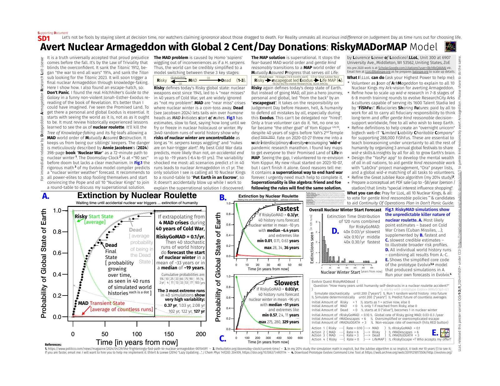
Figure 3: The SD1 poster. Full model code, simulation results, and MAP escape path on a single page. Download: SD1.#
To reproduce the results:
Download the Evolvix prototype compiler from Evolvix Prototype Compiler — Download and RiskyMAD Model Code
Enter the model code from Section 2.4 (or from the SD1 poster)
Run stochastic simulations
Compare your results with the published forecasts
The code is public. The compiler is public. The results are public. #AuditTheMath
9. Companion Papers#
The formal argument of Sections 2–4 is self-contained. The companion papers below provide the axiomatic framework from which these concepts were derived. They are recommended but not required for understanding the risk model or the MAP escape.
Upstream (b11–b15 provide the full formal context):
Matheo-b11 (b11, PET): Formal panentheistic axiom system. Divine experience varies with the world’s state (th4).
Matheo-b12 (b12, e7Day): Self-correcting construction model. BABL/ZION bifurcation (th3), OSCR collapse (m6.th1), Compassion Capacity.
Matheo-b13 (b13, e7He): Hero journey as anti-BABL inoculation. Commitment Trichotomy (th6), Supervillain Theorem.
Matheo-b14 (b14, JUB): Innovation theodicy, the Jubilee System (ax25), Binary Attractor theorem (th8).
Matheo-b15 (b15, Structural Deadlock): Divine Simplicity critique. Why ax11 (dipolarity) is necessary.
The PET connection, and what it is not. If divine experience covaries with the world’s state (th4 of Matheo-b11), then accidental nuclear winter affects the divine experience. Within this series’ framework the connection runs through Hartshorne’s dipolar theism: the stochastic certainty result is an existential risk for the concrete divine experience (contingent pole) while having no effect on the abstract divine nature (necessary pole).
It would be a mistake to call this “load-bearing” — and equally a mistake to pretend it played no part. The resolution is the same one Section 4.0a reaches about the remedy, and it is worth stating in the same words: a theological motivation removed a disincentive to measure; it did not supply the measurement. PET is why the author looked. It is not why the number is what it is. Nothing in Sections 2–4 depends on any claim in b11, and a reader who rejects the entire theological framework should find the forecast unchanged — that is the test, and the secular reading exists to make it easy to run.
Downstream:
Matheo-b17 (b17, h* Theorem): Falsifiable predictions. Who executes the plan? How to test whether they are genuine?
Matheo-b18 (b18, Call to Action): Synthesis. Includes the COOP (Continuity of Operations Plan) for the MAD → MAP transition.
10. Conclusion#
This paper set out to do one thing: put a waiting time on accidental nuclear winter, from the historical record, with every step open to inspection. Four results follow, and the first is the only one that needs to survive.
The comparison holds everywhere, including where it is attacked from every side at once. Death by accidental nuclear winter is more likely than death by a car crash, for most people — annual, per person, mortality against mortality. This is not a claim about the base case. It holds across every scenario in Table 3, and at the most optimistic corner it still stands at eighteen times the global road-death baseline. That corner is not a concession invented for this paper: it is the rate implied by the most sceptical published reading of the record (Section 5.3). The paper’s central claim survives its strongest critic’s own numbers — and survives, threefold, a simultaneous stress test in which that critic’s rate, the lowest published death fraction, and the road-death rate of the worst-affected country on record are applied together (Section 2.6). No figure here is offered as invariant. The inequality is.
The forecast is a bounded range, not a point. The annual probability that accidental nuclear winter begins lies between roughly 1 and 8 percent, with a base case of 2.90 percent — about 1 in 34 — calibrated from four Cuba-grade excursions in the forty Cold-War years, counted from someone else’s dataset under criteria fixed before counting. The mean time to onset is 30 years at the base rate and the median is 21 — half of all runs of world history are over inside 21 years. Over a forty-year horizon — one career — the base case gives 73 percent. The simulations and the arithmetic agree (Section 2.5): forty runs of world history returned a median near 19 years and roughly one blow-up in the first year, against exact values of 21.1 years and 1.16 per forty — both within sampling noise. The arithmetic does not overturn the simulations; it measures the same thing more finely, and reads slightly worse. Earlier formulations of “at least 1 in 40” hold at the base and pessimistic rates and over-state only at the optimistic corner. The single claim that does not survive is that 1-in-40 held regardless of scenario — it never did, and it was never a result of this model.
Danger
This paper corrects itself, in this paper’s own favour’s disfavour, and says so where a reader will see it. The immediately preceding draft computed its headline one-year probability with an exponential approximation while calling it exact. The true first-passage law is hypoexponential (Section 2.4a). The error ran to about 12 percent, in the direction that flattered the thesis, in the one number a reader is most likely to quote. It was found by the authors, before submission, and is reported in Section 2.0a rather than quietly repaired. A paper whose only request is that others check its arithmetic has no standing to make that request until it has checked its own.
The quiet years prove less than they appear to. The mechanism (Section 2.7) is a saturating two-step scheme of exactly the Michaelis–Menten form, and the world sits ninety times below half-saturation: the system is in its bound, lethal state about one percent of the time. A process like that produces long calm stretches as a matter of course. In the base scenario the median wait is 21 years, and yet the chance of surviving past 127 is 1.5 percent — not negligible, and one of the forty simulated runs did exactly that. Both are the same model. Eighty-one years without nuclear war is therefore weak evidence about the rate, which is precisely what makes the intuition “nothing has happened, so it cannot be that bad” so durable, and so unreliable.
The bottleneck is not arithmetic, and it is not ignorance either. That nuclear war would be catastrophic is among the most widely known facts on Earth. What is missing is narrower: a waiting-time distribution, in a form someone can act on. Baum’s survey concludes that nuclear war policy decisions “have made little use of risk analysis”, and that “the limiting factor is mainly the use of risk analysis for decision-making” [Baum, 2018]. Section 4.0 argues why, and the argument implicates this paper’s own author rather than exempting him: risks without visible remedies do not get measured, and measurements without visible remedies do not get used. Someone with the background, the motive, the tools, and a three-state model still took years to compute it. Section 6 reports what happened when he then tried to deliver it, and the finding there is not that anyone refused to listen. It is that there is no channel — which is the third defining feature of a super wicked problem [Lazarus, 2009] [Levin et al., 2012], operating exactly as specified.
What to do about that is Section 4’s business, and this paper does not claim to have settled it. What it claims is narrower and harder to dismiss: that the number is computable, that it has been computed here from public data by a method a competent reader can repeat in an afternoon, and that the answer is not small.
The only request this paper makes
Every input is public. The dataset is Baum, de Neufville and Barrett’s. The equations are in Section 2.4a, and the first-passage law is derived rather than assumed. The classification is in Tables 1 and 2, incident by incident, so that a reader who disagrees with a call can strike it and recompute — and the paper states in advance which two calls are weakest (Section 7.1b), which parameter is softest (Section 7.3), and what happens when the most contested incident is removed: 1 in 46 rather than 1 in 34.
Don’t believe it — #AuditTheMath. If the model is wrong, the fastest way to find out is for someone to check it and say so. That is a better outcome than being right.
References#
Barrett, A. M., Baum, S. D., & Hostetler, K. (2013). Analyzing and reducing the risks of inadvertent nuclear war between the United States and Russia. Science & Global Security, 21(2), 106–133. URL: https://scienceandglobalsecurity.org/archive/sgs21barrett.pdf, doi:10.1080/08929882.2013.798984
Barrett, A. M., Baum, S. D., & Hostetler, K. (2013). Appendix and supplement to “Analyzing and Reducing the Risks of Inadvertent Nuclear War between the United States and Russia”. Science & Global Security, 21(2). Online appendix to Barrett, Baum, and Hostetler (2013). URL: https://scienceandglobalsecurity.org/archive/sgs21barrett_app.pdf
Baum, S. D. (2018). Garrick, B. J. (Ed.). Reflections on the risk analysis of nuclear war. Proceedings of the Workshop on Quantifying Global Catastrophic Risks (pp. 19–50). Los Angeles, CA: Garrick Institute for the Risk Sciences, University of California, Los Angeles. https://gcri.org/publications/research/reflections-risk-analysis-nuclear-war.
Baum, S. D., de Neufville, R., & Barrett, A. M. (2018). A Model for the Probability of Nuclear War. Global Catastrophic Risk Institute. Working Paper 18-1, 8 March 2018. https://gcri.org/publications/research/model-probability-nuclear-war/.
Diaz-Maurin, F., & Mecklin, J. (2026). AI for peace: in Rome, Nobel laureates call for disarming AI and nuclear weapons. Bulletin of the Atomic Scientists. Bulletin of the Atomic Scientists, 17 July 2026. Available at https://thebulletin.org/2026/07/ai-for-peace-in-rome-nobel-laureates-call-for-disarming-ai-and-nuclear-weapons/. Reports the Global Nobel Laureates Assembly on Artificial Intelligence and Nuclear War, convened at the Vatican (Castel Gandolfo), 14–16 July 2026. URL: https://thebulletin.org/2026/07/ai-for-peace-in-rome-nobel-laureates-call-for-disarming-ai-and-nuclear-weapons/
Hellman, M. E. (2008). Risk analysis of nuclear deterrence. The Bent of Tau Beta Pi, 99(2), 14–22. URL: https://www.tbp.org/pubs/Features/Sp08Hellman.pdf
Hellman, M. E. (2021). Scouras, J. (Ed.). Probabilistic risk assessment. On Assessing the Risk of Nuclear War (pp. 85–126). Laurel, MD: The Johns Hopkins University Applied Physics Laboratory. Chapter 4. https://www.jhuapl.edu/sites/default/files/2022-12/Ch4_Hellman.pdf.
Korda, M., Johns, E., Knight-Boyle, M., & Kristensen, H. M. (2026 , February). The Aftermath: The Expiration of New START and What It Means For Us All. Federation of American Scientists.
Lazarus, R. J. (2009). Super wicked problems and climate change: restraining the present to liberate the future. Cornell Law Review, 94(5), 1153–1234. URL: https://scholarship.law.cornell.edu/clr/vol94/iss5/8/
Levin, K., Cashore, B., Bernstein, S., & Auld, G. (2012). Overcoming the tragedy of super wicked problems: constraining our future selves to ameliorate global climate change. Policy Sciences, 45(2), 123–152. URL: https://doi.org/10.1007/s11077-012-9151-0, doi:10.1007/s11077-012-9151-0
Lewis, P., Williams, H., Pelopidas, B., & Aghlani, S. (2014). Too Close for Comfort: Cases of Near Nuclear Use and Options for Policy. Chatham House (The Royal Institute of International Affairs). Chatham House Report, April 2014. https://www.chathamhouse.org/2014/04/too-close-comfort-cases-near-nuclear-use-and-options-policy.
Loewe, L., Scheuer, K. S., Keel, S. A., & others. (2017). Evolvix BEST names for semantic reproducibility across code2brain interfaces. Annals of the New York Academy of Sciences, 1387(1), 124–144. URL: https://doi.org/10.1111/nyas.13192, doi:10.1111/nyas.13192
Tertrais, B. (2017). “On The Brink”—really? Revisiting nuclear close calls since 1945. The Washington Quarterly, 40(2), 51–66. URL: https://doi.org/10.1080/0163660X.2017.1328922, doi:10.1080/0163660X.2017.1328922
Xia, L., Robock, A., Scherrer, K., Harrison, C. S., Bodirsky, B. L., Weindl, I., … Heneghan, R. (2022). Global food insecurity and famine from reduced crop, marine fishery and livestock production due to climate disruption from nuclear war soot injection. Nature Food, 3(8), 586–596. URL: https://doi.org/10.1038/s43016-022-00573-0, doi:10.1038/s43016-022-00573-0
Guinness World Records (2013). Deadliest Place to Travel by Road. Guinness World Records, "Deadliest place to travel by road": Libya, 73.4 road-traffic deaths per 100,000 (2013), citing the WHO Global Status Report on Road Safety 2015. Available at https://www.guinnessworldrecords.com/world-records/deadliest-place-to-travel-by-road.
International Campaign to Abolish Nuclear Weapons (2024). The Holy See and the Treaty on the Prohibition of Nuclear Weapons. Available at https://www.icanw.org/holy_see.
International Campaign to Abolish Nuclear Weapons (2026). The Expiration of New START: What It Means and What's Next. Available at https://www.icanw.org/new_start_expiration.
National Highway Traffic Safety Administration (2024). Traffic Safety Facts: 2023 Motor Vehicle Crashes — Overview. Available at https://www.nhtsa.gov/data/crash-data-systems.
Nobel Laureate Assembly for the Prevention of Nuclear War (2025). Declaration for the Prevention of Nuclear War. Nobel Laureate Assembly for the Prevention of Nuclear War, Chicago, July 2025. Available at https://nobelassembly.org/declaration/; full text at https://nobelassembly.org/declaration-for-the-prevention-of-nuclear-war-final/.
U.S. Government Accountability Office (2008). Terrorism Insurance: Status of Coverage Availability for Attacks Involving Nuclear, Biological, Chemical, or Radiological Weapons. U.S. Government Accountability Office. GAO-09-39, U.S. Government Accountability Office, 12 December 2008. Available at https://www.gao.gov/products/gao-09-39; full report PDF at https://www.gao.gov/assets/gao-09-39.pdf.
World Health Organization (2015). Global Status Report on Road Safety 2015. World Health Organization. World Health Organization, Geneva, 2015 (ISBN 978-92-4-156506-6; published 16 October 2015). Reports Libya's road-traffic death rate at 73.4 per 100,000 (2013 data), the highest national rate in the report. Available at https://www.who.int/publications/i/item/9789241565066; full PDF at https://iris.who.int/bitstream/handle/10665/189242/9789241565066_eng.pdf.
World Health Organization (2023). Global Status Report on Road Safety 2023. World Health Organization.
World Health Organization (2023). Road Safety: Libya 2023 Country Profile. Available at https://www.who.int/publications/m/item/road-safety-lby-2023-country-profile; country data at https://data.who.int/countries/434.